Some Tricks for Deep Learning in Complex Dynamical Systems Stuart - PDF document

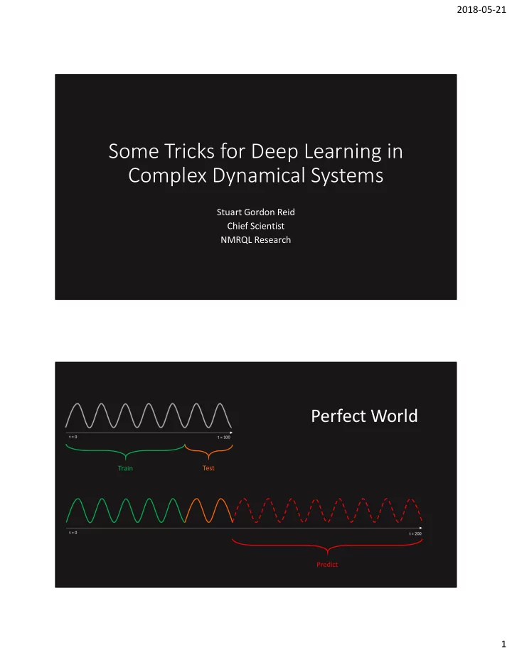
2018-05-21 Some Tricks for Deep Learning in Complex Dynamical Systems Stuart Gordon Reid Chief Scientist NMRQL Research Perfect World 1 t = 0 t = 100 Train Test 1 t = 0 t = 200 Predict 1

2018-05-21 t = 0 t = 100 Concept drift Regime change Phase transitions Error The Real World Most machine learning methods assume that the data generating process is stationary … This is quite often an unsound assumption 2

2018-05-21 Sensor degradation Sensor degradation caused by normal wear and tear or damage to mechanical equipment can result in significant changes to the distribution and quality of input and response data. Brand new, shiny, latest tech Aging, still shiny, yesterdays Fixed up after ‘minor’ damage with 100% working sensors tech with ~85% okay sensors with ~70% okay sensors Dynamical systems Other systems are inherently nonstationary, these are called dynamical systems . They can be stochastic, adaptive, or just sensitive to initial conditions. Examples include, but are not limited to: Habitats and ecosystems Weather systems Financial markets 3

2018-05-21 Data sampling The first set of ‘tricks’ involve how to sample data to train our deep learning model on Nonstationary (changing) environment 𝑢 + 2 𝑢 + 1 𝑢 4

2018-05-21 Supervised deep learning through time Our model learns a function which can map some set of input patterns, 𝐽 ���,� , to some set output responses, 𝑃 ���,� . In this setting there is it is assumed that the relationship between 𝐽 and 𝑃 is stationary over the window so there is one 𝑔 to approximate. The choice of window size (how much historical data to train the model on) poses a problem as it can be either optimistic or pessimistic. transfer knowledge + noise transfer knowledge + noise Fixed window size get 𝐽 � � and 𝑃 � � get 𝐽 � � and 𝑃 � � get 𝐽 � � and 𝑃 � � - Pessimistic data sampling + Adapts to change quickly 𝑥 � 𝑥 � 𝑥 � - Less data to train on + Faster (less data) - Inefficient data usage - Hard with large models transfer knowledge + noise transfer knowledge + noise Increasing window size get 𝐽 � � and 𝑃 � � get 𝐽 � � and 𝑃 � � get 𝐽 � � and 𝑃 � � - Optimistic data sampling - Adapts to change slowly 𝑥 � 𝑥 � 𝑥 � + More data to learn from - Slower (more data) - Most data is irrelevant ~ poor model performance 5

2018-05-21 Static ensemble over fixed window sizes To remove the choice of window size, we could try to construct a performance-weighted ensemble of models with different windows. The assumption here being that the model with the most relevant window size will perform the best out-of-sample. This is reasonable. The challenge with this approach is that it increases computational complexity which, in some dynamic environments, is infeasible. Static ensemble over different 𝑥 � 𝑥 � 𝑥 � window sizes get 𝐽 � � and 𝑃 � � get 𝐽 � � and 𝑃 � � get 𝐽 � � and 𝑃 � � ± Mixed and pessimistic and optimistic sampling transfer knowledge + noise transfer knowledge + noise ± Mixed fast and slow training 𝜁 + predictions 𝜁 + predictions 𝜁 + predictions times (more & less data) + Can adapt to change quickly - Increased computational complexity and runtime 𝜁 + predictions 𝜁 + predictions 𝜁 + predictions transfer knowledge + noise transfer knowledge + noise get 𝐽 � � and 𝑃 � � get 𝐽 � � and 𝑃 � � get 𝐽 � � and 𝑃 � � 𝑥 � 𝑥 � 𝑥 � 6

2018-05-21 Change detection & Hypothesis tests Another option is to try and determine the optimal window size using change detection tests and chained hypothesis tests. Change detection tests are typically done on some cumulative random variable (means, variances, spectral densities, errors, etc.). Hypothesis tests measure how likely two sequences of data have been sampled from the same distribution. It directly tests for stationarity. Change detected when some cumulative variable crosses a threshold estimated from Hoeffding bounds, Hellinger Change detection tests distance, or Kullback–Leibler divergence + A first principled approach to optimal window sizing + Computationally efficient + Neither optimistic not pessimistic if CDT and HT results are correct 𝜁 𝜁 𝜁 𝜁 𝜁 𝜁 𝜁 𝜁 𝜁 𝜁 𝜁 𝜁 𝜁 + Adapts to change when change occurs, otherwise transfer knowledge + noise transfer knowledge + noise just improves decisions - Sensitive to CDT threshold get 𝐽 � � and 𝑃 � � get 𝐽 � � and 𝑃 � � get 𝐽 � � and 𝑃 � � and p-values in HT 𝑥 � 𝑥 � 𝑥 � 7

2018-05-21 Time series subsequence clustering Another approach is to see the entire history of a given time series as an unsupervised classification problem and to use clustering methods. The goal is to cluster historical subsequence's (windows) into distinct clusters based on specific statistical characteristics of the sequences. One good old fashioned approach is to use k nearest neighbours. The only challenge can be the assignment of labels through time. transfer knowledge + noise Time series subsequence clustering model transfer knowledge + noise + Also a first principles approach to data sampling get 𝐽 � � and 𝑃 � � + Neither optimistic nor 𝑥 � 𝑥 � 𝑥 � pessimistic if clustering is correct / good enough + Data need not be sampled contiguously (NB!). - Sensitive to performance of the clustering algorithm - Computationally expensive and practically difficult. 0,1 1,0 1,0 1,0 0,1 0,1 1,0 0,1 0,1 8

2018-05-21 Data augmentation The second set of tricks involve how we can augment and Improve the data we have sampled to improve learning Data generation A challenge of pessimistic fixed window sizes and optimal window size estimation is not having enough data in the selected window. If the relevant window contains too few patterns then training large complex models becomes infeasible (they won’t converge). One approach to dealing with this problem is to train a simple generator and use it to amplify the training data for larger models. 9

2018-05-21 Data Generation transfer knowledge + noise transfer knowledge + noise + Enough data to fix complex get { 𝐽 � � } and { 𝑃 � � } get { 𝐽 � � } and { 𝑃 � � } get { 𝐽 � � } and { 𝑃 � � } models esp. RL agents - Still pessimistic data usage (can be overcome {𝑥 � , 𝑥 �∗ , … , 𝑥 �∗ } {𝑥 � , 𝑥 �∗ , … , 𝑥 �∗ } {𝑥 � , 𝑥 �∗ , … , 𝑥 �∗ } with CDT & HT tests) - Generator could easily produce nonsense if the data is too noisy or the generator is too simple. transfer knowledge + noise transfer knowledge + noise Not too different to 𝐻 𝐻 𝐻 + It’s pretty dope Doing a Monte Carlo Simulation except that The data is not random 𝑥 � 𝑥 � 𝑥 � Cluster (similarity) based sample weighting The time series clustering approach is equivalent to setting the ‘importance’ or sample weight of patterns sampled from clusters other than the one we are in to 0 and those from the cluster we are in to 1. This can be made more robust by measuring the probability of the most recent data points belonging to any given cluster and then weighting the patterns according those probabilities. 10

2018-05-21 Sample weighted time series subsequence clustering transfer knowledge + noise transfer knowledge + noise + Also a first principles approach to data sampling get 𝐽 � � and 𝑃 � � + Neither optimistic not 𝑥 � 𝑥 � 𝑥 � pessimistic if clustering is correct / good enough + Relevant needs not be sampled contiguously. + Less sensitive to performance of the clustering algorithm 0,1 1,0 1,0 0,1 0,1 1,0 0,1 0,1 + No need to keep different 1,0 models for different clusters just add more noise if the cluster changes (sees all) Neural network boosting ** Once we have sampled our data, we can further improve upon our selection by weighting the importance of patterns in that data. Boosting can be modified to ‘work around’ change points. This is done by initially weighting recent patterns higher than older patterns and then weighting easier patterns higher than harder patterns. The assumption here is that the hardest patterns will be those which are least similar to recent patterns so they should be down weighted. 11

2018-05-21 Neural network boosting 𝑥 � 𝑥 � 𝑥 � get 𝐽 � � and 𝑃 � � get 𝐽 � � and 𝑃 � � get 𝐽 � � and 𝑃 � � + Neural network can learn where patterns start to differ from recent ones. transfer knowledge + noise transfer knowledge + noise + Delicate balance between 𝜁 + predictions 𝜁 + predictions 𝜁 + predictions weighting and difficulty - Computationally expensive 𝜁 + predictions 𝜁 + predictions 𝜁 + predictions transfer knowledge + noise transfer knowledge + noise get 𝐽 � � and 𝑃 � � get 𝐽 � � and 𝑃 � � get 𝐽 � � and 𝑃 � � 𝑥 � 𝑥 � 𝑥 � Model augmentation The third set of tricks involve modifications to the model which allow it to adapt to change faster in 12