Some topological properties a b of planar lambda terms f g Noam - - PowerPoint PPT Presentation

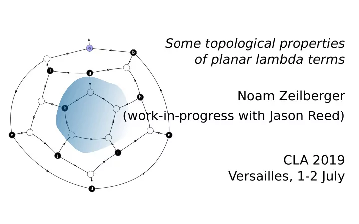
Some topological properties

• f planar lambda terms

CLA 2019 Versailles, 1-2 July Noam Zeilberger (work-in-progress with Jason Reed)

e f j k g d i b h c a

[Background]

A few views on maps

T

• pological definition

map = 2-cell embedding of a graph into a surface* considered up to deformation of the underlying surface.

*All surfaces are assumed to be connected and oriented throughout this talk

3 1 11 2 7 6 9 4 5 12 8 10

Algebraic definition

map = transitive permutation representation of the group considered up to G-equivariant isomorphism. G =

Combinatorial definition

map = connected graph + cyclic ordering of the half-edges around each vertex (say, as given by a drawing with "virtual crossings").

11 12 10 7 9 8 6 4 5 3 1 2 3 1 11 2 7 6 9 4 5 12 8 10

Graph versus Map ≡ ≢ ≡

graph map

≡

graph map

Some special kinds of maps

planar bridgeless 3-valent

Four Colour Theorem

The 4CT is a statement about maps.

every bridgeless planar map has a proper face 4-coloring

By a well-known reduction (T ait 1880), 4CT is equivalent to a statement about 3-valent maps

every bridgeless planar 3-valent map has a proper edge 3-coloring

Map enumeration

From time to time in a graph-theoretical career one's thoughts turn to the Four Colour Problem. It occurred to me once that it might be possible to get results of interest in the theory of map-colourings without actually solving the Problem. For example, it might be possible to find the average number of colourings on vertices, for planar triangulations of a given size. One would determine the number of triangulations of 2n faces, and then the number of 4-coloured triangulations of 2n faces. Then one would divide the second number by the first to get the required

• average. I gathered that this sort of retreat from a difficult problem to

a related average was not unknown in other branches of Mathematics, and that it was particularly common in Number Theory.

• W. T. T

utte, Graph Theory as I Have Known It

One of his insights was to consider rooted maps T utte wrote a pioneering series of papers (1962-1969)

• W. T. T

utte (1962), A census of planar triangulations. Canadian Journal of Mathematics 14:21–38

• W. T. T

utte (1962), A census of Hamiltonian polygons. Can. J. Math. 14:402–417

• W. T. T

utte (1962), A census of slicings. Can. J. Math. 14:708–722

• W. T. T

utte (1963), A census of planar maps. Can. J. Math. 15:249–271

• W. T. T

utte (1968), On the enumeration of planar maps. Bulletin of the American Mathematical Society 74:64–74

• W. T. T

utte (1969), On the enumeration of four-colored maps. SIAM Journal on Applied Mathematics 17:454–460

Key property: rooted maps have no non-trivial automorphisms

Map enumeration

Ultimately, T utte obtained some remarkably simple formulas for counting different families of rooted planar maps.

Map enumeration

[Background]

A few views on linear & planar λ-calculus

λx.λy.λz.x(yz) λx.λy.λz.(xz)y x,y ⊢ (xy)(λz.z) x,y ⊢ x((λz.z)y) λx.λy.λz.x(yz) λx.λy.λz.(xz)y x,y ⊢ (xy)(λz.z) x,y ⊢ x((λz.z)y)

pure lambda terms may be naturally organized into a cartesian operad

Untyped lambda calculus in modern dress

• Λ(n) = set of α-equivalence classes of linear terms in context x₁,...,xₙ ⊢ t
• ∘ᵢ : Λ(m+1) × Λ(n) → Λ(m+n) defined by (linear) substitution
• symmetric action Sₙ × Λ(n) → Λ(n) defined by permuting the context

linear terms may be naturally organized into an ordinary (symmetric) operad

(cf. Hyland, "Classical lambda calculus in modern dress")

x ⊢ x Γ, x ⊢ t Γ ⊢ λx.t Γ ⊢ t Δ ⊢ u Γ, Δ ⊢ t u Γ,y,x,Δ ⊢ t Γ,x,y,Δ ⊢ t Θ ⊢ u Γ,x,Δ ⊢ t Γ,Θ,Δ ⊢ t[u/x]

The operad of linear terms also has some natural suboperads:

• the non-symmetric operad of ordered ("planar") terms

Ordered & unitless terms

• the non-unitary operad of terms with no closed subterms (unitless/"bridgeless")

(Can also combine these two restrictions.) λx.λy.λz.x(yz) but not λx.λy.λz.(xz)y x ⊢ λy.yx but not x ⊢ x(λy.y)

Linear typing

typed linear terms may be interpreted as morphisms of a closed multicategory

x : A ⊢ x : A Γ, x : A ⊢ t : B Γ ⊢ λx.t : A ⊸ B Γ ⊢ t : A ⊸ B Δ ⊢ u : A Γ, Δ ⊢ t u : B

(technically, to get a closed multicategory we need to quotient by βη) the typed and untyped views are closely related...

• 1. every linear term can be typed
• 2. Λ is isomorphic to the endomorphism operad of a reflexive object

(NB: multicategory = colored operad)

reflexive object in a closed (2-)category

Idea (after D. Scott): a linear lambda term may be interpreted as an endomorphism of a reflexive object in a (symmetric) closed category. By a "reflexive object", we mean an object U equipped with a pair of operations

app

which need not compose to the identity. Actually, it is natural to work in a closed 2-category and ask that these operations witness an adjunction from U to U ⊸ U. Then the unit and the counit of this adjunction respectively interpret η-expansion t ⇒ λx.t(x) and β-reduction (λx.t)(u) ⇒ t[u/x].

lam

λ-graphs as string diagrams

A compact closed (2-)category is a particular kind of closed (2-)category in which A ⊸ B ≈ B ⊗ A*. There are many natural examples, such as Rel, the (2-)category of sets and relations.

λ @

Compact closed categories have a well-known graphical language of "string diagrams". By expressing reflexive objects in this language, we recover the traditional diagram representing a linear term (cf. George's talk).

string diagrams as HOAS

Another way of putting this is that these diagrams are closely related to the representation of λ-terms using higher-order abstract syntax

lam λx.lam λy.lam λz.app x (app y z) λx.λy.app (app x y)(lam λz.z)

[Background]

Enumera- & bijective connections

family of rooted maps family of lambda terms sequence OEIS

trivalent maps (genus g≥0) planar trivalent maps bridgeless trivalent maps bridgeless planar trivalent maps maps (genus g≥0) planar maps bridgeless maps bridgeless planar maps linear terms

• rdered terms

unitless linear terms unitless ordered terms normal linear terms (mod ~) normal ordered terms normal unitless linear terms (mod ~) normal unitless ordered terms A062980 A002005 A267827 A000309 A000698 A000168 A000699 A000260 1,5,60,1105,27120,... 1,4,32,336,4096,... 1,2,20,352,8624,... 1,1,4,24,176,1456,... 1,2,10,74,706,8162,... 1,2,9,54,378,2916,... 1,1,4,27,248,2830,... 1,1,3,13,68,399,...

• 1. O. Bodini, D. Gardy, A. Jacquot (2013), Asymptotics and random sampling for BCI and BCK lambda terms, TCS 502: 227-238
• 2. Z, A. Giorgetti (2015), A correspondence between rooted planar maps and normal planar lambda terms, LMCS 11(3:22): 1-39
• 3. Z (2015), Counting isomorphism classes of beta-normal linear lambda terms, arXiv:1509.07596
• 4. Z (2016), Linear lambda terms as invariants of rooted trivalent maps, J. Functional Programming 26(e21)
• 5. J. Courtiel, K. Yeats, Z (2016), Connected chord diagrams and bridgeless maps, arXiv:1611.04611
• 6. Z (2017), A sequent calculus for a semi-associative law, FSCD

family of rooted maps family of lambda terms sequence OEIS

trivalent maps (genus g≥0) planar trivalent maps bridgeless trivalent maps bridgeless planar trivalent maps maps (genus g≥0) planar maps bridgeless maps bridgeless planar maps linear terms

• rdered terms

unitless linear terms unitless ordered terms normal linear terms (mod ~) normal ordered terms normal unitless linear terms (mod ~) normal unitless ordered terms A062980 A002005 A267827 A000309 A000698 A000168 A000699 A000260 1,5,60,1105,27120,... 1,4,32,336,4096,... 1,2,20,352,8624,... 1,1,4,24,176,1456,... 1,2,10,74,706,8162,... 1,2,9,54,378,2916,... 1,1,4,27,248,2830,... 1,1,3,13,68,399,...

• 1. O. Bodini, D. Gardy, A. Jacquot (2013), Asymptotics and random sampling for BCI and BCK lambda terms, TCS 502: 227-238
• 2. Z, A. Giorgetti (2015), A correspondence between rooted planar maps and normal planar lambda terms, LMCS 11(3:22): 1-39
• 3. Z (2015), Counting isomorphism classes of beta-normal linear lambda terms, arXiv:1509.07596
• 4. Z (2016), Linear lambda terms as invariants of rooted trivalent maps, J. Functional Programming 26(e21)
• 5. J. Courtiel, K. Yeats, Z (2016), Connected chord diagrams and bridgeless maps, arXiv:1611.04611
• 6. Z (2017), A sequent calculus for a semi-associative law, FSCD

Some enumerative connections Some enumerative connections

Some enumerative connections

family of rooted maps family of lambda terms sequence OEIS

trivalent maps (genus g≥0) planar trivalent maps bridgeless trivalent maps bridgeless planar trivalent maps maps (genus g≥0) planar maps bridgeless maps bridgeless planar maps linear terms

• rdered terms

unitless linear terms unitless ordered terms normal linear terms (mod ~) normal ordered terms normal unitless linear terms (mod ~) normal unitless ordered terms A062980 A002005 A267827 A000309 A000698 A000168 A000699 A000260 1,5,60,1105,27120,... 1,4,32,336,4096,... 1,2,20,352,8624,... 1,1,4,24,176,1456,... 1,2,10,74,706,8162,... 1,2,9,54,378,2916,... 1,1,4,27,248,2830,... 1,1,3,13,68,399,...

• 1. O. Bodini, D. Gardy, A. Jacquot (2013), Asymptotics and random sampling for BCI and BCK lambda terms, TCS 502: 227-238
• 2. Z, A. Giorgetti (2015), A correspondence between rooted planar maps and normal planar lambda terms, LMCS 11(3:22): 1-39
• 3. Z (2015), Counting isomorphism classes of beta-normal linear lambda terms, arXiv:1509.07596
• 4. Z (2016), Linear lambda terms as invariants of rooted trivalent maps, J. Functional Programming 26(e21)
• 5. J. Courtiel, K. Yeats, Z (2016), Connected chord diagrams and bridgeless maps, arXiv:1611.04611
• 6. Z (2017), A sequent calculus for a semi-associative law, FSCD

Some enumerative connections

family of rooted maps family of lambda terms sequence OEIS

trivalent maps (genus g≥0) planar trivalent maps bridgeless trivalent maps bridgeless planar trivalent maps maps (genus g≥0) planar maps bridgeless maps bridgeless planar maps linear terms

• rdered terms

unitless linear terms unitless ordered terms normal linear terms (mod ~) normal ordered terms normal unitless linear terms (mod ~) normal unitless ordered terms A062980 A002005 A267827 A000309 A000698 A000168 A000699 A000260 1,5,60,1105,27120,... 1,4,32,336,4096,... 1,2,20,352,8624,... 1,1,4,24,176,1456,... 1,2,10,74,706,8162,... 1,2,9,54,378,2916,... 1,1,4,27,248,2830,... 1,1,3,13,68,399,...

• 1. O. Bodini, D. Gardy, A. Jacquot (2013), Asymptotics and random sampling for BCI and BCK lambda terms, TCS 502: 227-238
• 2. Z, A. Giorgetti (2015), A correspondence between rooted planar maps and normal planar lambda terms, LMCS 11(3:22): 1-39
• 3. Z (2015), Counting isomorphism classes of beta-normal linear lambda terms, arXiv:1509.07596
• 4. Z (2016), Linear lambda terms as invariants of rooted trivalent maps, J. Functional Programming 26(e21)
• 5. J. Courtiel, K. Yeats, Z (2016), Connected chord diagrams and bridgeless maps, arXiv:1611.04611
• 6. Z (2017), A sequent calculus for a semi-associative law, FSCD

From linear terms to rooted 3-valent maps via string diagrams

λx.λy.λz.x(yz) λx.λy.λz.(xz)y x,y ⊢ (xy)(λz.z) x,y ⊢ x((λz.z)y)

From linear terms to rooted 3-valent maps via string diagrams

λx.λy.λz.x(yz) λx.λy.λz.(xz)y x,y ⊢ (xy)(λz.z) x,y ⊢ x((λz.z)y)

From linear terms to rooted 3-valent maps via string diagrams

λx.λy.λz.x(yz) λx.λy.λz.(xz)y x,y ⊢ (xy)(λz.z) x,y ⊢ x((λz.z)y)

Observation: any rooted 3-valent map must have one of the following forms.

T1 T2 T1

disconnecting root vertex connecting root vertex no root vertex

From rooted 3-valent maps to linear terms by induction

...but this exactly mirrors the inductive structure of linear lambda terms!

application abstraction variable

T1 T2 T1

From rooted 3-valent maps to linear terms by induction

An example

An example

connecting

An example

An example

An example

An example

disconnecting

An example

An example

λa.λb.λc.λd.λe.a(λf.c(e(b(df))))

Some more examples*

*computed with the help of https://jcreedcmu.github.io/demo/lambda-map-drawer/public/index.html

λabcde.a (λfg.b (λh.c (λi.d (λj.e (f (λk.g (h (i (j k)))))))))

Some more examples*

*computed with the help of https://jcreedcmu.github.io/demo/lambda-map-drawer/public/index.html

λabcdefghi.a (λjk.b (λlm.(λno.c (λp.d (λq.e (λr.n (o (p (q r))))))) (λst.f (λu.g (λv.h (λw.s (t (u (v w))))))) (λx.i (j (k l (m x))))))

Some more examples*

*computed with the help of https://jcreedcmu.github.io/demo/lambda-map-drawer/public/index.html

λabcdefghijklm.a (λn.c (λopqr.(λstuv.d (λw.e (g ((λx.s (λy.t (v (n (b o) p (y u)))) (j (l x)) k) m (w f))))) (λz.h (i (q z) r))))

Some more analysis

planar ↔ ordered bridgeless ↔ unitless the bijection 3-valent maps ↔ linear terms restricts to the suboperads typing corresponds to edge-coloring (cf. JFP 2016, LICS 2018) ...indeed, there is a natural λ-formulation of 4CT!

• p

• p

β

3-valent map linear lambda term principal typing 𝕎-typing

• p

β

Connectivity in λ-calculus

[work-in-progress]

a graph is k-edge-connected if it stays connected after cutting any j < k edges 1-edge-connected = connected 2-edge-connected = bridgeless a 3-valent graph cannot be 4-edge-connected, but it can be internally 4-edge-connected (only trivial 3-cuts).

k-edge-connection

what does it mean for a linear λ-term to be internally k-edge-connected?

a term which is 2- but not 3-edge-connected

a,b ⊢ λc.a (λd.(b c) d)

*visualized with the help of https://www.georgejkaye.com/pages/fyp/visualiser.html

a,b ⊢ λc.a (λd.(b c) d)

a 3-edge-connected term

a,b ⊢ λc.a (λd.b (c d))

*visualized with the help of https://www.georgejkaye.com/pages/fyp/visualiser.html

A cut is a decomposition

towards a general definition

This definition gets a lot more interesting if we represent terms using HOAS and allow subterms to have higher type. We say that the type of a cut t = C{u} is the type of u.

• f a term t into a subterm u together with its surrounding context C.

Roughly speaking, a "context" is just a term with a hole/metavariable.

t = C{u}

towards a general definition

t : U ⊸ (U ⊸ U) t = λa.λb.lam λc.app a (lam λd.app (app b c) d) u : U ⊸ U u = λx.lam λd.app x d C : (U ⊸ U) ⇒ (U ⊸ (U ⊸ U)) C = {X}λa.λb.lam λc.app a (X (app b c))

For example, a few slides ago, we saw a term with a cut of type U ⊸ U a,b ⊢ λc.a (λd.b (c d))

towards a general definition

t : U t = lam λa.lam λb.lam λc. app a (lam λd.lam λe.lam λf. app (app b (app c d)) (app e f)) u₁ : (U ⊸ U) ⊸ U u₁ = λG.lam λe.lam λf.G (app e f) C₁ : (U ⊸ U) ⊸ U ⇒ U C₁ = {X}lam λa.lam λb.lam λc. app a (lam λd. X (λy.app (app b (app c d)) y))

Here is an example of a term with a yellow cut of type (U ⊸ U) ⊸ U and a blue cut of type U ⊸ (U ⊸ U) λa.λb.λc.a (λd.λe.λf.(b (c d)) (e f))

u₂ : U ⊸ (U ⊸ U) u₂ = λb.λc.lam λd.lam λe.lam λf. app (app b (app c d)) (app e f)) C₂ : U ⊸ (U ⊸ U) ⇒ U C₂ = {X}lam λa.lam λb.lam λc. app a (X b c)

A term is said to be k-indecomposable if it does not have any non-trivial τ-cuts where τ is a type with j < k occurrences of "U".

towards a general definition

The elementary terms are as follows: A cut t = C{u} is said to be trivial if either C is the identity or u is elementary.

λx.x app lam : U ⊸ U : U ⊸ (U ⊸ U) : (U ⊸ U) ⊸ U

Claim: t is k-indecomposable iff t is internally k-edge-connected.

3-indecomposable planar terms are counted by A000260, which also counts β-normal 2-indecomposable (= unitless) planar terms. Indeed, 3-indecomposable planar terms admit a direct inductive characterization...

results & questions

t C ::= x | C{t} ::= λx.C | • u

isomorphic to a similar characterization of β-normal unitless planar terms. Conjecture: β-normal 3-indecomposable planar terms are counted by A000257! What about non-planar 3-indecomposable terms?

results & questions

Q: Is there a direct inductive construction of 4-indecomposable planar terms? Theorem (T utte 1962): 4-indecomposable planar terms are counted by A000256 Theorem (Whitney 1931): every 4-indecomposable planar terms has a Hamiltonian cycle on its faces Q: Is there a λ-calculus proof of Whitney's theorem?