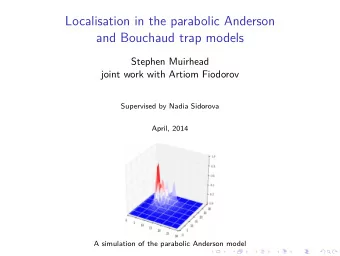
Some estimates for the parabolic Anderson model Samy Tindel Purdue - PowerPoint PPT Presentation

Some estimates for the parabolic Anderson model Samy Tindel Purdue University Probability Seminar - Urbana Champaign 2015 Collaborators: Xia Chen, Yaozhong Hu, Jingyu Huang, Khoa Lê, David Nualart Samy T. (Purdue) Parabolic Anderson model UIUC 2015 1 / 32

Outline Introduction 1 Motivations Aim of the talk Main results 2 Elements of proof 3 Samy T. (Purdue) Parabolic Anderson model UIUC 2015 2 / 32

Outline Introduction 1 Motivations Aim of the talk Main results 2 Elements of proof 3 Samy T. (Purdue) Parabolic Anderson model UIUC 2015 3 / 32

Some (recent) history Philip Anderson: Born 1923 Wide range of achievements ֒ → In condensed matter physics Contribution to Higgs mechanism Nobel prize in 1977 Still Professor at Princeton One of Anderson’s discoveries: For particles moving in a disordered media ֒ → Localized behavior instead of diffusion. Samy T. (Purdue) Parabolic Anderson model UIUC 2015 4 / 32

Equation under consideration Equation: Stochastic heat equation on R d : ∂ t u t , x = 1 2∆ u t , x + u t , x ˙ W t , x , (1) with t ≥ 0, x ∈ R d . ˙ W general Gaussian noise, with space-time covariance structure. u t , x ˙ W t , x differential: Stratonovich or Skorohod sense. Samy T. (Purdue) Parabolic Anderson model UIUC 2015 5 / 32

Outline Introduction 1 Motivations Aim of the talk Main results 2 Elements of proof 3 Samy T. (Purdue) Parabolic Anderson model UIUC 2015 6 / 32

Motivation 1: Resolution of SPDEs More general equation: ∂ t u t , x = Lu t , x + G ( u t , x ) + F ( u t , x ) ˙ W t , x , with General elliptic operator L Polynomial nonlinearity G Smooth nonlinearity F Samy T. (Purdue) Parabolic Anderson model UIUC 2015 7 / 32

Resolution of SPDEs (2) Resolution, Brownian W : Peszat-Zabczyk Dalang Resolution, rough paths case: Caruana-Friz-Oberhauser Lejay, Gubinelli-T, Gubinelli-T, Deya-Gubinelli-T Hairer Links: KPZ equation (Gubinelli-Perkowski, Hairer, Zambotti) Filtering, backward equations, stochastic control (Friz et al.) Question: Can we say more about u in the simple bilinear case u t , x ˙ W t , x ? Samy T. (Purdue) Parabolic Anderson model UIUC 2015 8 / 32

Motivation 2: Intermittency 2 ∆ u t , x + λ u t , x ˙ Equation: ∂ t u t , x = 1 W t , x Phenomenon: The solution u concentrates its energy in high peaks. Characterization: through moments ֒ → Easy possible definition of intermittency: for all k 1 > k 2 ≥ 1 � � E 1 / k 1 | u t , x | k 1 lim E 1 / k 2 [ | u t , x | k 2 ] = ∞ . t →∞ Results: White noise in time: Khoshnevisan, Foondun, Conus, Joseph Fractional noise in time: Balan-Conus Analysis through Feynman-Kac formula Samy T. (Purdue) Parabolic Anderson model UIUC 2015 9 / 32

Intemittency: illustration (by Daniel Conus) Simulations: for λ = 0 . 1, 0 . 5, 1 and 2. u(t,x) u(t,x) x x t t u(t,x) u(t,x) x x t t Samy T. (Purdue) Parabolic Anderson model UIUC 2015 10 / 32

Motivation 3: Polymer measure Independent Wiener measure: d -dimensional Brownian motion B x , Wiener measure P B . � t Hamiltonian for t > 0: − H t ( B x ) = 0 W ( ds , B x s ). Gibbs polymer measure: for β > 0, t ( B ) = e − β H t ( B x ) dG x d P B . u t , x Studies in the continuous case: Rovira-T, Lacoin, Alberts-Khanin-Quastel. Counterpart of intermittency: Localization. ֒ → See Carmona-Hu, König-Lacoin-Mörters-Sidorova Samy T. (Purdue) Parabolic Anderson model UIUC 2015 11 / 32

Localization: illustration 1 Figure: Simple random walk distribution Samy T. (Purdue) Parabolic Anderson model UIUC 2015 12 / 32

Localization: illustration 2 Figure: Distribution of the directed polymer in strong disorder regime Samy T. (Purdue) Parabolic Anderson model UIUC 2015 13 / 32

Motivation: summary Homogenization Pathwise PDEs 2 ∆ u + u ˙ ∂ t u = 1 Polymers W KPZ Intermittency � Local times Samy T. (Purdue) Parabolic Anderson model UIUC 2015 14 / 32

Outline Introduction 1 Motivations Aim of the talk Main results 2 Elements of proof 3 Samy T. (Purdue) Parabolic Anderson model UIUC 2015 15 / 32

Aim of the talk Equation: Stochastic heat equation on R d : ∂ t u t , x = 1 2∆ u t , x + u t , x ˙ W t , x . Main issues: for a general Gaussian noise, Resolution for Itô-Skorohod and Stratonovich equations. Feynman-Kac representation. Links between Feyman-Kac and pathwise (rough paths) solution. Intermittency estimates. Samy T. (Purdue) Parabolic Anderson model UIUC 2015 16 / 32

Outline Introduction 1 Motivations Aim of the talk Main results 2 Elements of proof 3 Samy T. (Purdue) Parabolic Anderson model UIUC 2015 17 / 32

Description of the noise Encoding the noise as a random distribution: W = { W ( ϕ ); ϕ ∈ H} centered Gaussian family E [ W ( ϕ ) W ( ψ )] = � ϕ, ψ � H with: � � ϕ, ψ � H = + × R 2 d ϕ ( s , x ) ψ ( t , y ) γ ( s − t ) Λ( x − y ) dx dy ds dt R 2 � = + × R d F ϕ ( s , ξ ) F ψ ( t , ξ ) γ ( s − t ) µ ( d ξ ) ds dt , R 2 γ , Λ positive definite functions. µ tempered measure. Remark: This is standard setting (Peszat-Zabczyk, Dalang). Samy T. (Purdue) Parabolic Anderson model UIUC 2015 18 / 32

Typical examples of noises Covariance Singularity at 0 FT: sing. at ∞ Roughness | t | − β B − β/ 2 γ ( t ) Not used B − 1 / 2 γ ( t ) δ ( t ) Not used � µ ( d ξ ) | x | − η B − η/ 2 Λ( x ) 1+ | ξ | η < ∞ R d Samy T. (Purdue) Parabolic Anderson model UIUC 2015 19 / 32

Possible solutions to the SHE Equation: ∂ t u t , x = 1 2∆ u t , x + u t , x ˙ W t , x , u 0 , x = u 0 ( x ) . Mild solution: � t � u t , x = p t u 0 ( x ) + R d p t − s ( x − y ) u s , y W ( ds , dy ) , 0 Feynman-Kac field: For a Brownian motion B independent of W , set � t � � t ) e V t , x � R d δ 0 ( B x u F u 0 ( B x V t , x = t − r − y ) W ( dr , dy ) , t , x = E B 0 Samy T. (Purdue) Parabolic Anderson model UIUC 2015 20 / 32

Stratonovich setting Hypothesis on γ : The function γ satisfies 0 ≤ γ ( t ) ≤ C β | t | − β , with β ∈ (0 , 1) . Hypothesis on µ : We assume the following integrability condition, � µ ( d ξ ) 1 + | ξ | 2 − 2 β < ∞ . R d Example: Riesz kernel in space, namely Λ( x ) = | x | − η . 0 < η ≤ 2 − 2 β . 0 ≤ γ ( t ) ≤ C β | t | − β . Samy T. (Purdue) Parabolic Anderson model UIUC 2015 21 / 32

Itô’s setting Dimension restriction: d = 1, that is x ∈ R ˙ Hypothesis on γ : W white noise in space, that is γ ( t ) = δ ( t ) Hypothesis on µ : for 1 / 4 < H < 1 / 2 (very rough situation), µ ( d ξ ) = | ξ | 1 − 2 H d ξ Samy T. (Purdue) Parabolic Anderson model UIUC 2015 22 / 32

Existence-uniqueness results Theorem 1. Existence-uniqueness, case 1: Under Stratonovich’s setting, Existence-uniqueness of a mild solution ֒ → In the rough paths (Young) sense. β 2 ([0 , T ]; B 1 − β ) Solution in C → B 1 − β weighted Besov space on R d . ֒ Existence-uniqueness, case 2: Under Itô’s setting, Existence-uniqueness of a mild solution ֒ → In the Itô sense. Solution in L 2 ([0 , T ]; B 1 / 2 − H ) Samy T. (Purdue) Parabolic Anderson model UIUC 2015 23 / 32

Feynman-Kac solution Theorem 2. Case 1: Under Stratonovich’s setting, Assume: u 0 ∈ C b ( R d ). B Brownian motion, independent of W We set (Feynman-Kac formula): � t � � t ) e V t , x � R d δ 0 ( B x u F u 0 ( B x V t , x = t − r − y ) W ( dr , dy ) , t , x = E B 0 Then u F well-defined and coincides with solution of SHE. Case 2: Under Itô’s setting ֒ → Feynman-Kac representation for moments Samy T. (Purdue) Parabolic Anderson model UIUC 2015 24 / 32

Moments estimates Theorem 3. Suppose: c 0 | t | − β ≤ γ ( t ) ≤ C 0 | t | − β . c 1 | x | − η ≤ Λ( x ) ≤ C 1 | x | − η . Then, whenever it is defined, u F satisfies: � � � � � � 4 − 2 β − η 4 − η 4 − 2 β − η 4 − η 2 − η k u k 2 − η k exp c 2 t ≤ E ≤ exp C 2 t . 2 − η 2 − η t , x Samy T. (Purdue) Parabolic Anderson model UIUC 2015 25 / 32

Growth rate Theorem 4. Under Itô’s setting, with 1 / 4 < H < 1 / 2 we have: � � 1 lim 1+ H ln | x |≤ R u ( t , x ) max = c H , 1 R →∞ [ln( R )] where c H is solution to a variational problem. Samy T. (Purdue) Parabolic Anderson model UIUC 2015 26 / 32

Comments Remarks: (i) Moment estimates imply intermittency. (ii) Important step: ֒ → exponential integrability of Feynman-Kac functional. (iii) Proof for moment estimates: ֒ → Feynman-Kac representation, small ball estimates. 1 (iv) Exponent 1+ H in growth rate: → extension of KPZ exponent 2 ֒ 3 for space-time white noise Extensions: (i) Extension 1: Non linear cases with σ ( u ) Lipschitz (ii) Extension 2: Skorohod (vs. Stratonovich) setting Samy T. (Purdue) Parabolic Anderson model UIUC 2015 27 / 32

Outline Introduction 1 Motivations Aim of the talk Main results 2 Elements of proof 3 Samy T. (Purdue) Parabolic Anderson model UIUC 2015 28 / 32