Some 0 / 1 polytopes need exponential size extended formulations - PowerPoint PPT Presentation
Some 0 / 1 polytopes need exponential size extended formulations Thomas Rothvo Department of Mathematics, M.I.T. b b b 0 / 1 polytopes conv( X ) with X { 0 , 1 } n P = (1 , 1) P (0 , 0) (1 , 0) b b b 0 / 1 polytopes conv( X ) with
Some 0 / 1 polytopes need exponential size extended formulations Thomas Rothvoß Department of Mathematics, M.I.T.
b b b 0 / 1 polytopes conv( X ) with X ⊆ { 0 , 1 } n P = (1 , 1) P (0 , 0) (1 , 0)
b b b 0 / 1 polytopes conv( X ) with X ⊆ { 0 , 1 } n P = → exponential! (1 , 1) P (0 , 0) (1 , 0)
b b b 0 / 1 polytopes conv( X ) with X ⊆ { 0 , 1 } n P = → exponential! { x ∈ R n | Ax ≤ b } = (1 , 1) P (0 , 0) (1 , 0)
b b b 0 / 1 polytopes conv( X ) with X ⊆ { 0 , 1 } n P = → exponential! { x ∈ R n | Ax ≤ b } = → exponential! (1 , 1) P (0 , 0) (1 , 0)
b b b 0 / 1 polytopes conv( X ) with X ⊆ { 0 , 1 } n P = → exponential! { x ∈ R n | Ax ≤ b } = → exponential! (1 , 1) P (0 , 0) (1 , 0)
b b b b b b b b b b b b b b b b b 0 / 1 polytopes conv( X ) with X ⊆ { 0 , 1 } n P = → exponential! { x ∈ R n | Ax ≤ b } = → exponential! = p ( Q ) → can be polynomial ◮ p : R n + k → R n linear projection ◮ Q = { ( x, y ) | Bx + Cy ≤ c } Q (1 , 1) P (0 , 0) (1 , 0)
b b b b b b b b b b b b b b b b b Extension complexity Definition Extension complexity: Q polyhedron xc( P ) := min #facets of Q | p linear projection p ( Q ) = P Q p P
b b b b b b b b b b b b b b b b b Extension complexity Definition Extension complexity: Q polyhedron xc( P ) := min #facets of Q | p linear projection p ( Q ) = P If xc( P ) ≤ poly ( n ) ⇒ ( Q, p ) compact formulation of P . Q p P
b b b b Example: Parity Polytope conv { x ∈ { 0 , 1 } n | # ones in x is odd } P = (0 , 1 , 1) (1 , 1 , 1) (1 , 0 , 1) (0 , 0 , 1) (0 , 1 , 0) (1 , 1 , 0) (0 , 0 , 0) (1 , 0 , 0)
b b b b Example: Parity Polytope conv { x ∈ { 0 , 1 } n | # ones in x is odd } P = = { 0 ≤ x ≤ 1 | x ( A ) − x ([ n ] \ A ) ≤ | A | − 1 ∀ A ⊆ [ n ] : | A | even } (0 , 1 , 1) (1 , 1 , 1) (1 , 0 , 1) (0 , 0 , 1) (0 , 1 , 0) (1 , 1 , 0) (0 , 0 , 0) (1 , 0 , 0)
b b b b Example: Parity Polytope conv { x ∈ { 0 , 1 } n | # ones in x is odd } P = = { 0 ≤ x ≤ 1 | x ( A ) − x ([ n ] \ A ) ≤ | A | − 1 ∀ A ⊆ [ n ] : | A | even } (0 , 1 , 1) (1 , 1 , 1) k = 3 k = 1 1 T z k (1 , 0 , 1) (0 , 0 , 1) = k ( k odd) 0 ≤ z k ≤ 1 (0 , 1 , 0) (1 , 1 , 0) (0 , 0 , 0) (1 , 0 , 0)
b b b b Example: Parity Polytope conv { x ∈ { 0 , 1 } n | # ones in x is odd } P = = { 0 ≤ x ≤ 1 | x ( A ) − x ([ n ] \ A ) ≤ | A | − 1 ∀ A ⊆ [ n ] : | A | even } (0 , 1 , 1) (1 , 1 , 1) � k = 3 z k x = k odd k = 1 1 T z k (1 , 0 , 1) (0 , 0 , 1) = k · λ k ( k odd) 0 ≤ z k ≤ 1 · λ k (0 , 1 , 0) (1 , 1 , 0) 1 T λ = 1 λ ≥ 0 (0 , 0 , 0) (1 , 0 , 0)
What’s known? Compact formulations: ◮ Perfect Matching in planar graphs [Barahona ’93] ◮ Perfect Matching in bounded genus graphs [Gerards ’91] ◮ O ( n log n )-size for Permutahedron [Goemans ’10] ( → tight ) ◮ n O (1 /ε ) -size ε -apx for Knapsack Polytope [Bienstock ’08] ◮ . . .
What’s known? Compact formulations: ◮ Perfect Matching in planar graphs [Barahona ’93] ◮ Perfect Matching in bounded genus graphs [Gerards ’91] ◮ O ( n log n )-size for Permutahedron [Goemans ’10] ( → tight ) ◮ n O (1 /ε ) -size ε -apx for Knapsack Polytope [Bienstock ’08] ◮ . . . Theorem (Yannakakis) No symmetric compact formulation for TSP Polytope and Perfect Matching Polytope .
What’s known? Compact formulations: ◮ Perfect Matching in planar graphs [Barahona ’93] ◮ Perfect Matching in bounded genus graphs [Gerards ’91] ◮ O ( n log n )-size for Permutahedron [Goemans ’10] ( → tight ) ◮ n O (1 /ε ) -size ε -apx for Knapsack Polytope [Bienstock ’08] ◮ . . . Theorem (Yannakakis) No symmetric compact formulation for TSP Polytope and Perfect Matching Polytope . Theorem (Kaibel, Pashkovich & Theis ’10) Compact formulation for log n size matchings, but no symmetric one.
1st Carg` ese Workshop on Combinatorial Optim.
1st Carg` ese Workshop on Combinatorial Optim.
1st Carg` ese Workshop on Combinatorial Optim.
1st Carg` ese Workshop on Combinatorial Optim.
1st Carg` ese Workshop on Combinatorial Optim. Open problem I Does the matching polytope have a compact formulation?
1st Carg` ese Workshop on Combinatorial Optim. Open problem I ! a e d Does the matching polytope i o N have a compact formulation?
1st Carg` ese Workshop on Combinatorial Optim. Open problem I ! a e d Does the matching polytope i o N have a compact formulation?
1st Carg` ese Workshop on Combinatorial Optim. Open problem I ! a e d Does the matching polytope i o N have a compact formulation? Open problem II (V. Kaibel) Is there any 0/1 polytope without a compact formulation?
1st Carg` ese Workshop on Combinatorial Optim. Open problem I ! a e d Does the matching polytope i o N have a compact formulation? Open problem II (V. Kaibel) ! s Is there any 0/1 polytope without e Y a compact formulation? Theorem For every n there exists X ⊆ { 0 , 1 } n s.t. xc(conv( X )) ≥ 2 n/ 2 · (1 − o (1)) .
Proof strategy X ⊆ { 0 , 1 } n
Proof strategy conv( X ) � �� � x | ∃ y : A x + B y ≤ b X ⊆ { 0 , 1 } n
Proof strategy injective conv( X ) � �� � map x | ∃ y : A x + B y ≤ b X ⊆ { 0 , 1 } n
Proof strategy injective conv( X ) � �� � map x | ∃ y : A x + B y ≤ b X ⊆ { 0 , 1 } n #0 / 1 polytopes ≤ # extended form.
Proof strategy injective conv( X ) � �� � map x | ∃ y : A x + B y ≤ b X ⊆ { 0 , 1 } n #0 / 1 polytopes ≤ # extended form. = 2 2 n
Proof strategy irrational entries injective conv( X ) � �� � map x | ∃ y : A x + B y ≤ b X ⊆ { 0 , 1 } n √ 2 #0 / 1 polytopes ≤ # extended form. = = 2 2 n ∞
Proof strategy irrational entries injective conv( X ) � �� � map x | ∃ y : A x + B y ≤ b X ⊆ { 0 , 1 } n ! k √ 2 r o w t #0 / 1 polytopes ≤ # extended form. ’ n s e = = o D 2 2 n ∞
Slack-matrix Write: P = conv( { x 1 , . . . , x v } ) = { x ∈ R n | Ax ≤ b } � �� � non-redundant # vertices Slack-matrix S S ij # facets S ij = b i − A T i x j
Slack-matrix Write: P = conv( { x 1 , . . . , x v } ) = { x ∈ R n | Ax ≤ b } � �� � non-redundant # vertices vertex Slack-matrix j S S ij facet i # facets S ij = b i − A T i x j
Slack-matrix Write: P = conv( { x 1 , . . . , x v } ) = { x ∈ R n | Ax ≤ b } � �� � non-redundant # vertices V ≥ 0 r r Slack-matrix S U ≥ S ij # facets S ij = b i − A T i x j 0 Non-negative rank: rk + ( S ) = min { r | ∃ U ∈ R f × r ≥ 0 , V ∈ R r × v ≥ 0 : S = UV }
Example for slack-matrix (1 , 1) 0 1 0 S x 1 − x 2 ≥ 0 2 x 1 ≤ 2 2 0 0 P 0 0 1 (0 , 0) x 2 ≥ 0 (1 , 0)
Yannakakis’ Theorem Theorem (Yannakakis ’91) Let S be slackmatrix for P : ◮ xc ( P ) = rk + ( S ) . ◮ For any non-neg. factorization S = UV : P = { x ∈ R n | ∃ y ≥ 0 : Ax + Uy = b }
Yannakakis’ Theorem Theorem (Yannakakis ’91) Let S be slackmatrix for P : ◮ xc ( P ) = rk + ( S ) . ◮ For any non-neg. factorization S = UV : P = { x ∈ R n | ∃ y ≥ 0 : Ax + Uy = b } ◮ For vertex x j : A i x j + U i V j = b i .
Yannakakis’ Theorem Theorem (Yannakakis ’91) Let S be slackmatrix for P : ◮ xc ( P ) = rk + ( S ) . ◮ For any non-neg. factorization S = UV : P = { x ∈ R n | ∃ y ≥ 0 : Ax + Uy = b } ◮ For vertex x j : A i x j + U i V j = b i . ◮ A i x > b i = ⇒ A i x + U i y > b i . ���� ≥ 0
Yannakakis’ Theorem Theorem (Yannakakis ’91) Let S be slackmatrix for P : ◮ xc ( P ) = rk + ( S ) . ◮ For any non-neg. factorization S = UV : P = { x ∈ R n | ∃ y ≥ 0 : Ax + Uy = b } ◮ For vertex x j : A i x j + U i V j = b i . ◮ A i x > b i = ⇒ A i x + U i y > b i . ���� ≥ 0 ◮ “ ≥ ” follows from an application of duality.
Controlling the coefficients ◮ Fix X ⊆ { 0 , 1 } n , P := conv( X ) = { x ∈ R n | Ax ≤ b } and Slack-matrix S = UV Valid assumption: ◮ A, b integral with � A � ∞ , � b � ∞ ≤ 2 n log(2 n )
Controlling the coefficients ◮ Fix X ⊆ { 0 , 1 } n , P := conv( X ) = { x ∈ R n | Ax ≤ b } and Slack-matrix S = UV Valid assumption: ◮ A, b integral with � A � ∞ , � b � ∞ ≤ 2 n log(2 n ) ◮ xc( P ) ≤ 2 n .
Controlling the coefficients ◮ Fix X ⊆ { 0 , 1 } n , P := conv( X ) = { x ∈ R n | Ax ≤ b } and Slack-matrix S = UV Valid assumption: ◮ A, b integral with � A � ∞ , � b � ∞ ≤ 2 n log(2 n ) ◮ xc( P ) ≤ 2 n . ◮ | S ij | = | b i − A i x j | ≤ ( n + 1) · 2 n log(2 n ) ≤ 2 n 2
Recommend
More recommend
Explore More Topics
Stay informed with curated content and fresh updates.
