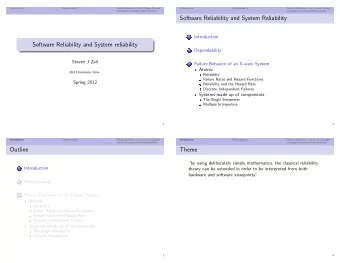
Software Reliability and System Reliability Recap 1 Historical - PowerPoint PPT Presentation

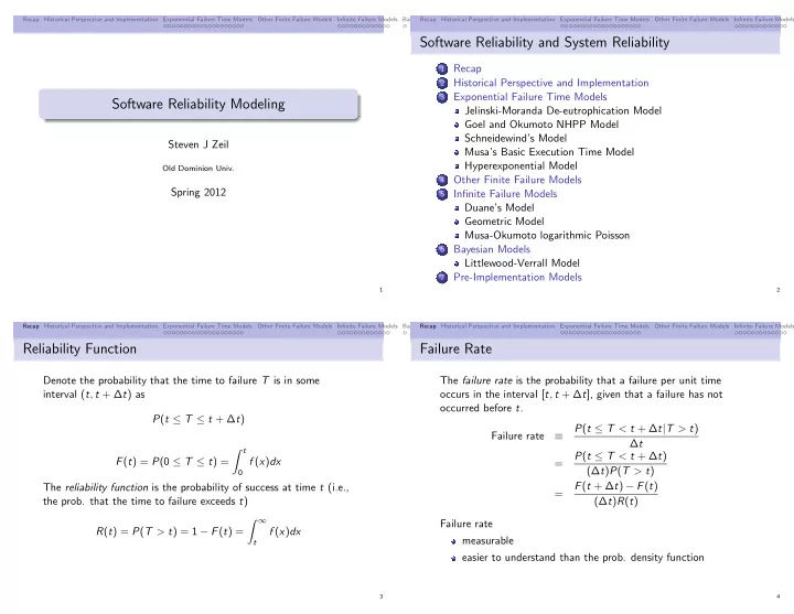
Recap Historical Perspective and Implementation Exponential Failure Time Models Other Finite Failure Models Infinite Failure Models Bayesian Models Recap Historical Perspective and Implementation Pre-Implementation Models Exponential Failure Time Models Other Finite Failure Models Infinite Failure Models Software Reliability and System Reliability Recap 1 Historical Perspective and Implementation 2 Exponential Failure Time Models 3 Software Reliability Modeling Jelinski-Moranda De-eutrophication Model Goel and Okumoto NHPP Model Schneidewind’s Model Steven J Zeil Musa’s Basic Execution Time Model Hyperexponential Model Old Dominion Univ. Other Finite Failure Models 4 Spring 2012 Infinite Failure Models 5 Duane’s Model Geometric Model Musa-Okumoto logarithmic Poisson Bayesian Models 6 Littlewood-Verrall Model Pre-Implementation Models 7 1 2 Recap Historical Perspective and Implementation Exponential Failure Time Models Other Finite Failure Models Infinite Failure Models Bayesian Models Recap Historical Perspective and Implementation Pre-Implementation Models Exponential Failure Time Models Other Finite Failure Models Infinite Failure Models Reliability Function Failure Rate Denote the probability that the time to failure T is in some The failure rate is the probability that a failure per unit time interval ( t , t + ∆ t ) as occurs in the interval [ t , t + ∆ t ], given that a failure has not occurred before t . P ( t ≤ T ≤ t + ∆ t ) P ( t ≤ T < t + ∆ t | T > t ) Failure rate ≡ ∆ t � t P ( t ≤ T < t + ∆ t ) F ( t ) = P (0 ≤ T ≤ t ) = f ( x ) dx = (∆ t ) P ( T > t ) 0 F ( t + ∆ t ) − F ( t ) The reliability function is the probability of success at time t (i.e., = the prob. that the time to failure exceeds t ) (∆ t ) R ( t ) � ∞ Failure rate R ( t ) = P ( T > t ) = 1 − F ( t ) = f ( x ) dx measurable t easier to understand than the prob. density function 3 4

Recap Historical Perspective and Implementation Exponential Failure Time Models Other Finite Failure Models Infinite Failure Models Bayesian Models Recap Historical Perspective and Implementation Pre-Implementation Models Exponential Failure Time Models Other Finite Failure Models Infinite Failure Models Hazard Rate Failure Intensity Function The hazard rate is defined as the limit of the failure rate as the � t � � interval ∆ t approaches zero. R ( t ) = exp − z ( x ) dx 0 F ( t + ∆ t ) − F ( t ) = f ( t ) or, differentiating z ( t ) = lim (∆ t ) R ( t ) Rt ∆ t → 0 � t � � The hazard rate is an instantaneous rate of failure at time t , given f ( t ) = z ( t ) exp − z ( x ) dx 0 that the system survives up to t . z ( t ) dt represents the probability that a system of age t will fail in the small interval t to t + dt . 5 6 Recap Historical Perspective and Implementation Exponential Failure Time Models Other Finite Failure Models Infinite Failure Models Bayesian Models Recap Historical Perspective and Implementation Pre-Implementation Models Exponential Failure Time Models Other Finite Failure Models Infinite Failure Models Relating Reliability to Failure Rate (2) Reliability and the Failure Intensity Alternatively, t e → 0 (1 − p ( t e )) t / t e = exp( − λ t ) Let t e be time required to execute one test case. R ( t ) = lim which is the exponential distribution t = kt e Assume that there is a finite limit for p / t e as t e becomes vanishingly small p λ = lim t e t e → 0 This is the failure intensity function . 7 8

Recap Historical Perspective and Implementation Exponential Failure Time Models Other Finite Failure Models Infinite Failure Models Bayesian Models Recap Historical Perspective and Implementation Pre-Implementation Models Exponential Failure Time Models Other Finite Failure Models Infinite Failure Models Data Faults and Failures Models typically employ In this chapter, no distinction is made between faults and failures. They are assumed to be 1-to-1. failures per time period, or Implies that we fix all faults before they have a chance to cause a time between failures 2nd failure. Conversion between the two is possible, with some caveats. Let M ( t ) be a random variable denoting the number of failures (faults) experienced by time t . Let µ ( t ) be the mean value function of M ( t ). 9 10 Recap Historical Perspective and Implementation Exponential Failure Time Models Other Finite Failure Models Infinite Failure Models Bayesian Models Recap Historical Perspective and Implementation Pre-Implementation Models Exponential Failure Time Models Other Finite Failure Models Infinite Failure Models Model Classification Scheme Poisson Processes Musa & Okumoto classify models according to The Poisson distribution describes the probability of a given number of events occurring in a fixed interval given that events 1 Time domain: wall clock versus execution time occur at a fixed rate and are independent of the time since the last 2 Category: total number of failures over infinite time event. What is lim t →∞ µ ( t )? f ( k ; λ ) = λ k e − λ finite k ! infinite Divide time range 0 . . . t into a sequence of observation points 3 Type: distribution of the number of failures experienced by t 0 , t 1 , . . . t n with t 0 = 0 and t n = t . time t Let f i denote the # of failures occurring in t i − 1 . . . t i . Poisson If the f i are independent Poisson variables, we have a Poisson binomial process. 4 Class (finite failure models only): Functional form of the failure intensity as a function of time E [ f i ] = µ ( t i ) − µ ( t i − 1 ) 5 Family (infinite failure models only): Functional form of the failure intensity as a function of expected number of failures experienced 11 12

Recap Historical Perspective and Implementation Exponential Failure Time Models Other Finite Failure Models Infinite Failure Models Bayesian Models Recap Historical Perspective and Implementation Pre-Implementation Models Exponential Failure Time Models Other Finite Failure Models Infinite Failure Models Reliability of a Poisson Process Poisson Process and Single Faults Let ∆ t be any non-negative value such that t i − 1 + ∆ t < t i . The the prob that the software will run reliably for another ∆ t z (∆ t | t i − 1 ) = λ ( t i − 1 + ∆ t ) given that it has not yet failed at t i − 1 is � t +∆ t µ ( t ) = α F a ( t ) � � R (∆ t | t ) = P ( f i = 0 | t ) = exp − λ ( x ) dx where α is the number of faults (as t → ∞ ) and F a ( t ) is the t cumulative distribution of the time to failure of a single fault a . λ ( t ) = α f a ( t ) 13 14 Recap Historical Perspective and Implementation Exponential Failure Time Models Other Finite Failure Models Infinite Failure Models Bayesian Models Recap Historical Perspective and Implementation Pre-Implementation Models Exponential Failure Time Models Other Finite Failure Models Infinite Failure Models Binomial Processes Exponential Failure Time Models Assume Models in which the failure intensity function λ ( t ) is exponential. Recap 1 N is the fixed, total number of faults in the system Historical Perspective and Implementation 2 Faults are removed immediately upon detection and new Exponential Failure Time Models 3 faults are never added Jelinski-Moranda De-eutrophication Model Goel and Okumoto NHPP Model If T a is a reandom variable denoting the time to failure of Schneidewind’s Model fault a , the T a ’s are i.i.d. Musa’s Basic Execution Time Model The F a ( t ), f a ( t ), and z a ( t ) are identical for all faults in this class. Hyperexponential Model Other Finite Failure Models 4 λ ( t ) = Nf a ( t ) Infinite Failure Models 5 µ ( t ) = NF a ( t ) Duane’s Model Geometric Model N in binomial process is similar to α in the Poisson with a single Musa-Okumoto logarithmic Poisson type of fault. Bayesian Models 6 Littlewood-Verrall Model Pre-Implementation Models 7 15 16