Software Quality Engineering: Testing, Quality Assurance, and - PDF document

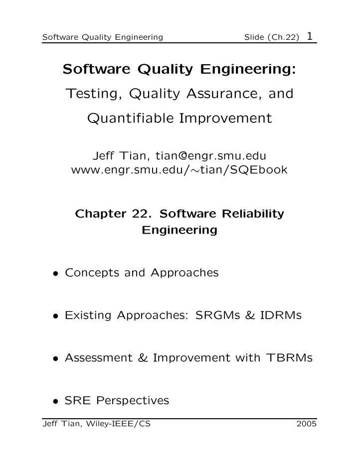
Slide (Ch.22) 1 Software Quality Engineering Software Quality Engineering: Testing, Quality Assurance, and Quantifiable Improvement Jeff Tian, tian@engr.smu.edu www.engr.smu.edu/ ∼ tian/SQEbook Chapter 22. Software Reliability Engineering • Concepts and Approaches • Existing Approaches: SRGMs & IDRMs • Assessment & Improvement with TBRMs • SRE Perspectives Jeff Tian, Wiley-IEEE/CS 2005

Slide (Ch.22) 2 Software Quality Engineering What Is SRE • Reliability: Probability of failure-free oper- ation for a specific time period or input set under a specific environment ⊲ Failure: behavioral deviations ⊲ Time: how to measure? ⊲ Input state characterization ⊲ Environment: OP • Software reliability engineering: ⊲ Engineering (applied science) discipline ⊲ Measure, predict, manage reliability ⊲ Statistical modeling ⊲ Customer perspective: – failures vs. faults – meaningful time vs. development days – customer operational profile Jeff Tian, Wiley-IEEE/CS 2005

Slide (Ch.22) 3 Software Quality Engineering Assumption: SRE and OP • Assumption 1: OP, to ensure software re- liability from a user’s perspective. • OP: Operational Profile ⊲ Quantitative characterization of the way a (software) system will be used. ⊲ Test case generation/selection/execution ⊲ Realistic assessment ⊲ Predictions (minimize discontinuity) • OP topics in SQE book: ⊲ Chapter 8: Musa’s OP – flat list with probabilities – tree-structured OP – dev. procedures: Musa-1/Musa-2 ⊲ Chapter 10: Markov chains and UMMs (unified Markov models) Jeff Tian, Wiley-IEEE/CS 2005

Slide (Ch.22) 4 Software Quality Engineering Other Assumptions in Context • Assumption 2: Randomized testing ⊲ Independent failure intervals/observations ⊲ Approximation in large software systems ⊲ Adjustment for non-random testing ⇒ new models or data treatments • Assumption 3: Failure-fault relation ⊲ Failure probability ∼ # faults ⊲ Exposure through OP-based testing ⊲ Possible adjustment? ⊲ Statistical validity for large s/w systems Jeff Tian, Wiley-IEEE/CS 2005

Slide (Ch.22) 5 Software Quality Engineering Other Assumptions and Context • Assumption 4: time-reliability relation ⊲ Time measurement in SRGMs ⊲ Usage-dependent vs. usage-independent ⊲ Proper choice under specific env. • Usage-independent time measurement: ⊲ Calendar/wall-clock time ⊲ Only if stable or constant workload • Usage-dependent time measurement: ⊲ Execution time – Musa’s models ⊲ Runs, transactions, etc. ⊲ Most systems with uneven workload e.g., Fig 22.1 & Fig 22.2 (pp.374-375) Jeff Tian, Wiley-IEEE/CS 2005

Slide (Ch.22) 6 Software Quality Engineering Input Domain Reliability Models • IDRMs: Current reliability snapshot based on observed testing data of n samples. • Assessment of current reliability. • Prediction of future reliability (limited prediction due to snapshot) • Management and improvement ⊲ As acceptance criteria. ⊲ Risk identification and followups: – reliability for input subsets – remedies for problematic areas – preventive actions for other areas Jeff Tian, Wiley-IEEE/CS 2005

Slide (Ch.22) 7 Software Quality Engineering Nelson’s IDRM • Nelson Model: ⊲ Running for a sample of n inputs. ⊲ Randomly selected from set E : E = { E i : i = 1 , 2 , . . . , N } ⊲ Sampling probability vector: { P i : i = 1 , 2 , . . . , N } ⊲ { P i } : Operational profile. ⊲ Number of failures: f . ⊲ Estimated reliability: n = n − f R = 1 − r = 1 − f n ⊲ Failure rate: r . • Repeated sampling without fixing. Jeff Tian, Wiley-IEEE/CS 2005

Slide (Ch.22) 8 Software Quality Engineering Other IDRMs and Applications • Brown-Lipow model: ⊲ Explicit input state distribution. ⊲ Known probability for sub-domains E i ⊲ f i failures for n i runs from subdomain E i N f i � R = 1 − P ( E i ) n i i =1 • Application examples ⊲ Nelson model for a large s/w system – succ. segments: Table 22.1 (p.376) ⊲ Nelson model for web applications – daily error rates: Table 22.2 (p.377) ⊲ Other models possible (Tian 2002) Jeff Tian, Wiley-IEEE/CS 2005

Slide (Ch.22) 9 Software Quality Engineering Time Domain Measures and Models • Reliability measurement ⊲ Reliability: time & probability ⊲ Result: failure vs. success ⊲ Time/input measurement ⊲ Failure intensity (rate): alternative ⊲ MTBF/MTTF: summary measure • S/w reliability growth models (SRGMs): ⊲ Reliability growth due to defect removal based on observed testing data. ⊲ Reliability-fault relations ⊲ Exposure assumptions ⊲ Data: time-between-failure (TBF) vs. period-failure-count (PFC) models Jeff Tian, Wiley-IEEE/CS 2005

Slide (Ch.22) 10 Software Quality Engineering Basic Functions (Time Domain) • Failure distribution functions: ⊲ F ( t ): cumulative distribution function (cdf) for failure over time ⊲ f ( t ): prob. density function (pdf) f ( t ) = F ′ ( t ) • Reliability-related functions: ⊲ Reliability function R ( t ) = 1 − F ( t ) R ( t ) = P ( T ≥ t ) = P (no failure by t ) ⊲ Hazard function/rate/intensity z ( t )∆ t = P { t < T < t + ∆ t | T > t } • Jelinski-Moranda (de-eutrophication) model: z i = φ ( N − ( i − 1)) Jeff Tian, Wiley-IEEE/CS 2005

Slide (Ch.22) 11 Software Quality Engineering Other Basic Definitions • MTBF, MTTF, and reliability ⊲ Mean time to failure (MTTF) � ∞ � ∞ MTTF = tf ( t ) dt = R ( t ) dt 0 0 ⊲ Mean time between failures (MTBF) = MTTF for memoryless process – similarly defined ⊲ good summary measure of reliability • Reliability-hazard relation: R ( t ) = e − � t 0 z ( x ) dx 1 − F ( t ) = f ( t ) f ( t ) z ( t ) = R ( t ) Jeff Tian, Wiley-IEEE/CS 2005

Slide (Ch.22) 12 Software Quality Engineering Other Basic Functions • Overall failure arrival process: (as compared to individual failures) • NHPP (non-homogeneous Poisson process): ⊲ Most commonly used for modeling ⊲ Probability of n failures in [0 , t ]: P ( N ( t ) = n ) = m ( t ) n e − m ( t ) n ! ⊲ m ( t ): mean function ⊲ Failure rate/intensity λ ( t ): λ ( t ) = m ′ ( t ) = dm ( t ) dt • Other processes: Binomial, etc. Jeff Tian, Wiley-IEEE/CS 2005

Slide (Ch.22) 13 Software Quality Engineering Commonly Used NHPP Models • Goel-Okumoto model m ( t ) = N (1 − e − bt ) – N : estimated # of defects – b : model curvature • S-shaped model: m ( t ) = N (1 − (1 + bt ) e − bt ) – allow for slow start – may be more descriptive • Musa-Okumoto execution time model: m ( τ ) = 1 θ log( λ 0 θτ + 1) – emphasis: execution time τ Jeff Tian, Wiley-IEEE/CS 2005

Slide (Ch.22) 14 Software Quality Engineering SRGM Applications • Assessment of current reliability • Prediction of future reliability and resource to reach reliability goals • Management and improvement ⊲ Reliability goals as exit criteria ⊲ Resource allocation (time/distribution) ⊲ Risk identification and followups: – reliability (growth) of different areas – remedies for problematic areas – preventive actions for other areas • Examples: Fig. 22.3 (p.380) and Section 22.4. Jeff Tian, Wiley-IEEE/CS 2005

Slide (Ch.22) 15 Software Quality Engineering Assessing Existing Approaches • Time domain reliability analysis: ⊲ Customer perspective. ⊲ Overall assessment and prediction. ⊲ Ability to track reliability change. ⊲ Issues: assumption validity. ⊲ Problem: how to improve reliability? • Input domain reliability analysis: ⊲ Explicit operational profile. ⊲ Better input state definition. ⊲ Hard to handle change/evolution. ⊲ Issues: sampling and practicality. ⊲ Problem: realistic reliability assessment? Jeff Tian, Wiley-IEEE/CS 2005

Slide (Ch.22) 16 Software Quality Engineering TBRMs: An Integrated Approach • Combine strengths of the two. • TBRM for reliability modeling: ⊲ Input state: categorical information. ⊲ Each run as a data point. ⊲ Time cutoff for partitions. ⊲ Data sensitive partitioning ⇒ Nelson models for subsets. • Using TBRMs: ⊲ Reliability for partitioned subsets. ⊲ Use both input and timing information. ⊲ Monitoring changes in trees. ⊲ Enhanced exit criteria. ⊲ Integrate into the testing process. Jeff Tian, Wiley-IEEE/CS 2005

Slide (Ch.22) 17 Software Quality Engineering TBRMs • Tree-based reliability models (TBRMs): TBM using all information. • Response: Result indicator r ij . ⊲ r ij = 1 for success, 0 for failure. ⊲ Nelson model for subsets: n i s i = 1 r ij = n i − f i = ˆ � or R i n i n i j =1 � n i � n i j =1 t ij s ij j =1 r ij = S i = ˆ s i = = R i . � n i � n i j =1 t j j =1 t j T i • Predictors: Timing and input states. ⊲ Data sensitive partitioning. ⊲ Key factors affecting reliability. Jeff Tian, Wiley-IEEE/CS 2005

Slide (Ch.22) 18 Software Quality Engineering TBRMs: Interpretation & Usage • Interpretation of trees: ⊲ Predicted response: success rate. (Nelson reliability estimate.) ⊲ Time predictor: reliability change. ⊲ State predictor: risk identification. • Change monitoring and risk identification: ⊲ Change in predicted response. ⊲ Through tree structural change. ⊲ Identify high risk input state. ⊲ Additional analyses often necessary. ⊲ Enhanced test cases or components. ⊲ Examples: Fig 22.4 and 22.5 (p.383). Jeff Tian, Wiley-IEEE/CS 2005