Smooth Constraint Convex Minimization via Conditional Gradients - - PowerPoint PPT Presentation

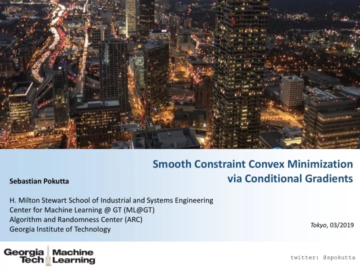
Sebastian Pokutta

• H. Milton Stewart School of Industrial and Systems Engineering

Center for Machine Learning @ GT (ML@GT) Algorithm and Randomness Center (ARC) Georgia Institute of Technology

twitter: @spokutta

Tokyo, 03/2019

Smooth Constraint Convex Minimization via Conditional Gradients

2

Joint Work with… (in random order)

Alexandre D’Aspremont Gábor Braun Thomas Kerdreux Swati Gupta Cyrille Combettes Robert Hildebrand Stephen Wright Yi Zhou George Lan Dan Tu Daniel Zink

3

(C (Constrain int) ) Co Convex Opti timiz izatio ion

Convex Optimization: Given a feasible region 𝑄 solve the optimization problem: Min𝑦∈𝑄 𝑔 𝑦 , where 𝑔 is a convex function (+ extra properties). Our setup.

• 1. Access to 𝑄. Linear Optimization (LO) oracle: Given linear objective c

𝑦 ← argmin𝑤∈𝑄𝑑𝑈𝑤

• 2. Access to 𝑔. First-Order (FO) oracle: Given 𝑦 return

𝛼𝑔 𝑦 and 𝑔(𝑦) => Complexity of convex optimization relative to LO/FO oracle

Source: [Jaggi 2013]

4

Why would ld you care for r constrain int convex opti timiz izatio ion?

Setup captures various problems in Machine Learning, e.g.:

• 1. OCR (Structured SVM Training)

1. Marginal polytope over chain graph of letters of word and quadratic loss

• 2. Video Co-Localization

1. Flow polytope and quadratic loss

• 3. Lasso

1. Scaled ℓ1-ball and quadratic loss (regression)

• 4. Regression over structured objects

1. Regression over convex hull of combinatorial atoms

• 5. Approximation of distributions

1. Bayesian inference, sequential kernel herding, …

5

Smooth Convex Optim imiz ization 101

6

Ba Basic ic noti tions

Let 𝑔: 𝑆𝑜 → 𝑆 be a function. We will use the following basic concepts:

• Smoothness. 𝑔 𝑧 ≤ 𝑔 𝑦 + ∇𝑔 𝑦 𝑈 𝑧 − 𝑦 +

𝑀 2 𝑦 − 𝑧 2

• Convexity. 𝑔 𝑧 ≥ 𝑔 𝑦 + ∇𝑔 𝑦 𝑈 𝑧 − 𝑦

Strong Convexity. 𝑔 𝑧 ≥ 𝑔 𝑦 + ∇𝑔 𝑦 𝑈 𝑧 − 𝑦 + 𝜈

2

𝑦 − 𝑧

2

=> Use for optimization unclear. Next step: Operationalize notions!

7

Mea easu sures of f Progr gress ss: Smooth thness and Id Idealized Gradient t Descent

Consider an iterative algorithm of the form: 𝑦𝑢+1 ← 𝑦𝑢 − 𝜃𝑢𝑒𝑢 By definition of smoothness. 𝑔 𝑦𝑢 − 𝑔 𝑦𝑢+1 ≥ 𝜃𝑢∇𝑔 𝑦𝑢 𝑈𝑒𝑢 − 𝜃𝑢

2 𝑀 2

𝑒𝑢

2

Smoothness induces primal progress. Optimizing right-hand side: 𝑔 𝑦𝑢 − 𝑔 𝑦𝑢+1 ≥ ∇𝑔 𝑦𝑢 𝑈𝑒𝑢 2 2𝑀 𝑒𝑢

2

for 𝜃𝑢∗ = ∇𝑔 𝑦𝑢 𝑈𝑒𝑢 𝑀 𝑒𝑢

2

Idealized Gradient Descent (IGD). Choose 𝑒𝑢 ← 𝑦𝑢 − 𝑦∗ (non-deterministic!) 𝑔 𝑦𝑢 − 𝑔 𝑦𝑢+1 ≥ ∇𝑔 𝑦𝑢 𝑈(𝑦𝑢 − 𝑦∗) 2 2𝑀 𝑦𝑢 − 𝑦∗

2

for 𝜃𝑢∗ = ∇𝑔 𝑦𝑢 𝑈(𝑦𝑢 − 𝑦∗) 𝑀 𝑦𝑢 − 𝑦∗

8

Measu sures of f Optim timality: Convexity ty

Recall convexity: 𝑔 𝑧 ≥ 𝑔 𝑦 + ∇𝑔 𝑦 𝑈 𝑧 − 𝑦 Primal bound from Convexity. 𝑦 ← 𝑦𝑢 and 𝑧 ← 𝑦∗ ∈ argmin𝑦∈𝑄𝑔 𝑦 : ℎ𝑢 ≔ 𝑔 𝑦𝑢 − 𝑔 𝑦∗ ≤ ∇𝑔 𝑦𝑢 𝑈(𝑦𝑢 − 𝑦∗) Plugging this into the progress from IGD and 𝑦𝑢 − 𝑦∗ ≤ 𝑦0 − 𝑦∗ . 𝑔 𝑦𝑢 − 𝑔 𝑦𝑢+1 ≥ ∇𝑔 𝑦𝑢 𝑈 𝑦𝑢 − 𝑦∗

2

2𝑀 𝑦𝑢 − 𝑦∗

2

≥ ℎ𝑢

2

2𝑀 𝑦0 − 𝑦∗

2

Rearranging provides contraction and convergence rate. ℎ𝑢+1 ≤ ℎ𝑢 ⋅ 1 − ℎ𝑢 2𝑀 𝑦0 − 𝑦∗

2

⇒ ℎ𝑈 ≤ 2𝑀 𝑦0 − 𝑦∗

2

𝑈 + 4

9

Measu sures of f Optim timality: Str trong Convexity ty

Recall strong convexity: 𝑔 𝑧 ≥ 𝑔 𝑦 + ∇𝑔 𝑦 𝑈 𝑧 − 𝑦 +

𝜈 2

𝑦 − 𝑧

2

Primal bound from Strong Convexity. 𝑦 ← 𝑦𝑢 and 𝑧 ← 𝑦𝑢 − 𝛿(𝑦𝑢 − 𝑦∗) ℎ𝑢 ≔ 𝑔 𝑦𝑢 − 𝑔 𝑦∗ ≤ ∇𝑔 𝑦𝑢 𝑈 𝑦𝑢 − 𝑦∗

2

2𝜈 𝑦𝑢 − 𝑦∗

2

Plugging this into the progress from IGD. 𝑔 𝑦𝑢 − 𝑔 𝑦𝑢+1 ≥ ∇𝑔 𝑦𝑢 𝑈 𝑦𝑢 − 𝑦∗

2

2𝑀 𝑦𝑢 − 𝑦∗

2

≥ 𝜈 𝑀 ℎ𝑢 Rearranging provides contraction and convergence rate. ℎ𝑢+1 ≤ ℎ𝑢 ⋅ 1 − 𝜈 𝑀 ⇒ ℎ𝑈 ≤ 𝑓−𝜈

𝑀𝑈 ⋅ ℎ0

10

From IG IGD to actu tual l alg lgorit ithms

Consider an algorithm of the form: 𝑦𝑢+1 ← 𝑦𝑢 − 𝜃𝑢𝑒𝑢 Scaling condition (Scaling). Show there exist 𝛽𝑢 with ∇𝑔 𝑦𝑢 𝑈𝑒𝑢 𝑒𝑢 ≥ 𝛽𝑢 ∇𝑔 𝑦𝑢 𝑈 𝑦𝑢 − 𝑦∗ 𝑦𝑢 − 𝑦∗ => Lose an 𝜷𝒖

𝟑 factor in iteration 𝒖. Bounds and rates follow immediately.

• Example. (Vanilla) Gradient Descent with 𝑒𝑢 ← ∇𝑔(𝑦𝑢)

∇𝑔 𝑦𝑢 𝑈𝑒𝑢 𝑒𝑢 = ∇𝑔 𝑦𝑢

2 ≥ 1 ⋅ ∇𝑔 𝑦𝑢 𝑈 𝑦𝑢 − 𝑦∗

𝑦𝑢 − 𝑦∗ => TODAY: No more convergences proofs. Just establishing (Scaling).

11

Conditional Gradients (a.k .k.a .a. Frank-Wolfe Alg lgorit ithm)

12

Co Condit itio ional l Gradie ients a.k .k.a. . Frank-Wolf lfe Alg lgorit ithm

• 1. Advantages

1. Extremely simple and robust: no complicated data structures to maintain 2. Easy to implement: requires only a linear optimization oracle (first order method) 3. Projection-free: feasibility via linear optimization oracle 4. Sparse distributions over vertices: optimal solution is convex comb. (enables sampling)

• 2. Disadvantages

1. Suboptimal convergence rate of 𝑃(

1 𝑈) in the worst-case

=> Despite suboptimal rate often used because of simplicity

Source: [Jaggi 2013]

13

Co Condit itio ional l Gradie ients a.k .k.a. . Frank-Wolf lfe Alg lgorit ithm

𝑦1 = 𝑤1 ) −∇𝑔(𝑦1) 𝑤2 𝑦2 −∇𝑔(𝑦2) 𝑤3 𝑦3

Note: A) Points are formed as convex combinations of vertices B) vertices used to write point => „Active sets“

14

Co Condit itio ional l Gradie ients a.k .k.a. . Frank-Wolf lfe Alg lgorit ithm

Establishing (Scaling). FW algorithm takes direction 𝑒𝑢 = 𝑦𝑢 − 𝑤𝑢. Observe ∇𝑔 𝑦 𝑈 𝑦𝑢 − 𝑤𝑢 ≥ ∇𝑔 𝑦 𝑈 𝑦𝑢 − 𝑦∗ Hence with 𝛽𝑢 =

| 𝑦𝑢−𝑦∗ | 𝐸

with D diameter of P: ∇𝑔 𝑦 𝑈 𝑦𝑢 − 𝑤𝑢 | 𝑦𝑢 − 𝑤𝑢 | ≥ 𝑦𝑢 − 𝑦∗ 𝐸 ⋅ ∇𝑔 𝑦 𝑈 𝑦𝑢 − 𝑦∗ 𝑦𝑢 − 𝑦∗ => This 𝜷𝒖 is sufficient for 𝑷(

𝟐 𝒖) convergence but better??

Source: [Jaggi 2013]

15

Th The str trongly convex case Lin inear convergence in in sp special cases

If 𝑔 is strongly convex we would expect a linear rate of convergence. Obstacle. ∇𝑔 𝑦 𝑈 𝑦𝑢 − 𝑤𝑢 | 𝑦𝑢 − 𝑤𝑢 | ≥ 𝒚𝒖 − 𝒚∗ 𝐸 ⋅ ∇𝑔 𝑦 𝑈 𝑦𝑢 − 𝑦∗ 𝑦𝑢 − 𝑦∗ Special case 𝑦∗ ∈ rel. int 𝑄 , say 𝐶 𝑦∗, 2𝑠 ⊆ 𝑄. Then: Theorem [Marcotte, Guélat ‘86]. After a few iterations ∇𝑔 𝑦 𝑈 𝑦𝑢 − 𝑤𝑢 | 𝑦𝑢 − 𝑤𝑢 | ≥ 𝑠 𝐸 ⋅ ∇𝑔 𝑦 𝑈 𝑦𝑢 − 𝑦∗ 𝑦𝑢 − 𝑦∗ and linear convergence follows via (Scaling).

16

Th The str trongly convex case Is Is lin linear convergence in in general poss ssible?

(Vanilla) Frank-Wolfe cannot achieve linear convergence in general: Theorem [Wolfe ‘70]. 𝑦∗ on boundary of P. For any 𝜀 > 0 for infinitely many t: 𝑔 𝑦𝑢 − 𝑔 𝑦∗ ≥ 1 𝑢1+𝜀 Issue: zig-zagging (b/c first order opt) [Wolfe ‘70] proposed Away Steps

17

Th The str trongly convex case Lin inear convergence in in general

First linear convergence result (in general) due to [Garber, Hazan ‘13]

• 1. Simulating (theoretically efficiently) a stronger oracle rather using Away Steps
• 2. Involved constants are extremely large => algorithm unimplementable

Linear convergence for implementable variants due to [Lacoste-Julien, Jaggi ‘15]

• 1. (Dominating) Away-steps are enough
• 2. Includes most known variants: Away-Step FW, Pairwise CG, Fully-Corrective FW,

Wolfe’s algorithm, …

• 3. Key ingredient: There exists 𝑥(𝑄) (depending on polytope 𝑄 (only!)) s.t.

∇𝑔 𝑦 𝑈 𝑏𝑢 − 𝑤𝑢 ≥ 𝑥 𝑄 ∇𝑔 𝑦 𝑈 𝑦𝑢 − 𝑦∗ 𝑦𝑢 − 𝑦∗ (𝑒𝑢 = 𝑏𝑢 − 𝑤𝑢 is basically the direction that either variant dominates) => Linear convergence via (Scaling)

18

Many more variants and results…

Recently there has been a lot of work on Conditional Gradients, e.g.,

• 1. Linear convergence for conditional gradient sliding [Lan, Zhou ‘14]
• 2. Linear convergence for (some) non-strongly convex functions [Beck, Shtern ‘17]
• 3. Online FW [Hazan, Kale ‘12, Chen et al ‘18]
• 4. Stochastic FW [Reddi et al ‘16] and Variance-Reduced Stochastic FW [Hazan,

Luo ’16, Chen et al ‘18]

• 5. In-face directions [Freund, Grigas ‘15]
• 6. Improved convergence under sharpness [Kerdreux, D’Aspremont, P. ‘18]

… and many more!! => Very competitive and versatile in real-world applications

19

Revis isit iting Conditional Gradie ients

20

Bottle tleneck 1: : Cost t of f Lin inear Optim timization Drawbacks s in in th the context t of f hard feasible regio gions

Basic assumption of conditional gradient methods: Linear Optimization is cheap As such accounted for as 𝑃(1). This assumption is not warranted if:

• 1. Linear Program of feasible region is huge

1. Large shortest path problems 2. Large scheduling problems 3. Large-scale learning problems

• 2. Optimization over feasible region is NP-hard

1. TSP tours 2. Packing problems 3. Virtually every real-world combinatorial optimization problem

21

Reth thin inkin ing CG in in th the context xt of f exp xpensiv ive oracle le calls lls

Basic assumption for us: Linear Optimization is not cheap (Think: hard IP can easily require an hour to be solved => one call/it unrealistic)

• 1. Questions:

1. Is it necessary to call the oracle in each iteration? 2. Is it necessary to compute (approximately) optimal solutions? 3. Can we reuse information?

• 2. Theoretical requirements

1. Achieve identical convergence rates, otherwise any speedup will be washed out

• 3. Practical requirements

1. Make as few oracle calls as possible

22

La Lazif ific icatio ion approach of f [B [BPZ 2017] usin sing weaker oracle le

• 1. Interpretation of Weak Separation Oracle: Discrete Gradient Directions

1. Either a new point 𝑧 ∈ 𝑄 that improves the current objective by at least

Φ 𝐿 (positive call)

2. Or it asserts that all other points 𝑨 ∈ 𝑄 improve no more than Φ (negative call)

• 2. Lazification approach of [Braun, P., Zink ‘17]

1. Use weaker oracle that allows for caching and early termination (no more expensive than LP) 2. Advantage: huge speedups in wall-clock time when LP is hard to solve 1. For hard LPs speedups can be as large as 107 3. Disadvantage: weak separation oracle produces even weaker approximations than LP oracle 1. Actual progress in iterations can be worse than with LP oracle 2. Advantage vanishes if LP is very cheap and can be actually worse than original algorithm 3. Caching is not “smart”: it simple iterates over the already seen vertices

• 3. Optimal complexity for Weak Separation Oracle [Braun, Lan, P., Zhou ‘17]

23

Bottle tleneck 2: : Quality ty of f gr gradient approximati tion Frank-Wolfe vs.

• s. Proje

jected Gradient t Desc scent

𝑦𝑢 −∇𝑔(𝑦𝑢) 𝑤1 𝑤2

Gradient Descent-style progress Problem: how far can we go into this direction without leaving the feasible region? Solution: do a gradient step and project back into feasible region. However can be very expensive

𝑦𝑢+1

Frank-Wolfe approach Use directions formed via vertices as approximations of the gradient and form convex combinations only. Problem: Approximations can be bad, i.e., 𝛂𝐠 𝐲𝐮 , 𝐰 − 𝐲𝐮 small

𝑤2 − 𝑦𝑢 𝑤1 − 𝑦𝑢 𝑦𝑢+1 = (1 − 𝜇)𝑦𝑢 + 𝜇𝑤1  Tradeoff between ensured feasibility and quality of gradient approximations!

24

Brin inging Conditional Gradients as clo lose as possible le to Gradie ient Descent

25

𝑦∗ 𝑤4 𝑦𝑢 𝑤2 𝑤1 𝑤3

Gradient Descent Phase As long as enough progress, perform gradient descent over the simplex (𝒘𝟐, 𝒘𝟑, 𝒘𝟒)

𝑦𝑢+𝑚

Frank-Wolfe Phase Once progress over simplex too small, call LP oracle to obtain new vertex and simplex

−∇𝑔(𝑦𝑢+𝑚) 𝑦𝑢+𝑚+1

Ble Blendin ing of f grad adie ient steps an and Fran ank-Wolf lfe steps

26

St Stayin ing Projec jectio ion-fr free: Th The Sim Simple lex Descent Oracle le (SiD SiDO)

• 1. Interpretation of Simplex Descent Oracle: Single progress step on simplex

1. Either reduce size of set 𝑇 by at least 1 if function is not increasing (guaranteed progress in size) 2. Or make a descent step with a guaranteed improvement relative to best approximate direction (guaranteed progress in function value)

• 2. Various implementations of SiDO

1. Most basic via projected gradient descent (PGD) however requires projections over a low- dimensional simplices 2. Better version via new(!!) projection-free algorithm over simplex (Simplex Gradient Descent) with cost linear in the size of the active set per iteration

27

Th The alg lgorit ithm: : Ble Blended Co Condit itio ional l Gradie ients

Frank-Wolfe Phase Once progress too small, call LPSep

• racle for new vertex and simplex

Gradient Descent Phase As long as enough progress, perform gradient descent over the simplex Dual Gap Update Phase If neither SiDO nor Frank-Wolfe steps can progress enough update dual gap

28

Main in Th Theorem

You basically get what you expect:

• Theorem. [Braun, P., Tu, Wright ‘18] Assume 𝑔 is convex and smooth over the

polytope 𝑄 with curvature 𝐷 and geometric strong convexity 𝜈. Then Algorithm 1 ensures: 𝑔 𝑦𝑢 − 𝑔 𝑦∗ ≤ 𝜁 for 𝑢 ≥ Ω 𝐷 𝜈 log Φ0 𝜁 , where 𝑦∗ is an optimal solution to 𝑔 over 𝑄 and Φ0 ≥ 𝑔 𝑦0 − 𝑔(𝑦∗). (For previous empirical work with similar idea see also [Rao, Shah, Wright ‘15])

29

Co Computatio ional l Resu sult lts

Lasso Structured Regression Sparse Signal Recovery Matrix Completion

30

Beyond Conditional Gradie ients: Ble lended Matchin ing Pursuit it

31

(G (Generali lized) Matchin ing Pursuit it

Special variant of constraint convex minimization: Given a set of vectors 𝒝 ⊆ 𝑆𝑜 solve: Minlin(𝒝) 𝑔 𝑦 , where 𝑔 is a convex function. Basic example: 𝑔

𝑧 𝑦 =

𝑦 − 𝑧

2

Source: [Locatello et al ‘17]

32

Ble lended (G (Generalized) ) Match ching Pursu suit t [Combettes, P. ‘19] Faster th than MP with ith sp sparsity ty of f OMP

Inspired by [Locatello et al 2017] same blending idea can be used for MP.

33

Interestingly, (unaccelerated) BGMP even outperforms accelerated MP as using actual gradient directions over FW approximations seem to offset acceleration.

Ble lended (G (Generalized) ) Match ching Pursu suit Faster th than MP with ith sp sparsity ty of f OMP

34

Co Code is is publi licly ly avail ilable le

Code available at: https://www.github.com/pokutta/bcg

• 1. Python package for Python 3.5+
• 2. Reasonably well optimized (work in progress…)
• 3. Automatic differentiation via autograd
• 4. Interfaces with gurobi

Trying to use autograd to compute gradient... Dimension of feasible region: 10 ╭──────────────┬──────────┬────────────────────────┬────────────────────────┬──────────────┬──────────────╮ │ Iteration │ Type │ Function Value │ Dual Bound │ #Atoms │ WTime │ ├──────────────┼──────────┼────────────────────────┼────────────────────────┼──────────────┼──────────────┤ │ 1 │ FI │ 3255589.0000000005 │ 6629696.0 │ 1 │ 0.0018 │ │ 2 │ FI │ 2590612.0 │ 6629696.0 │ 2 │ 0.0036 │ │ 3 │ FN │ 2565368.125 │ 6629696.0 │ 2 │ 0.0053 │ │ 4 │ P │ 2560989.662200928 │ 178146.5 │ 2 │ 0.0071 │ │ 5 │ P │ 2559806.0614284277 │ 178146.5 │ 2 │ 0.0085 │ │ 6 │ P │ 2559680.2272379696 │ 178146.5 │ 2 │ 0.0103 │ │ 7 │ P │ 2559538.3483599476 │ 178146.5 │ 2 │ 0.0126 │ │ 8 │ FI │ 2538950.9169786745 │ 178146.5 │ 3 │ 0.0141 │ │ 9 │ PD │ 2499078.142760788 │ 178146.5 │ 2 │ 0.0164 │ │ 10 │ P │ 2376118.39724563 │ 178146.5 │ 2 │ 0.0175 │ │ 11 │ FN │ 2375260.49557375 │ 178146.5 │ 2 │ 0.0187 │ │ 12 │ FN │ 2375259.67380736 │ 28354.22443160368 │ 2 │ 0.0206 │ │ 13 │ FN │ 2375259.6279250253 │ 1093.4857637005916 │ 2 │ 0.0235 │ │ 14 │ FN │ 2375259.627728738 │ 201.47828699820093 │ 2 │ 0.0255 │ │ 15 │ FN │ 2375259.62771675 │ 16.927091718331212 │ 2 │ 0.0273 │ │ 16 │ FN │ 2375259.6277167373 │ 3.2504734088724945 │ 2 │ 0.0298 │ │ 17 │ FN │ 2375259.6277167364 │ 0.13467991727520712 │ 2 │ 0.0321 │ │ 18 │ FN │ 2375259.627716736 │ 0.02344177945633419 │ 2 │ 0.0343 │ │ 19 │ FN │ 2375259.627716736 │ 0.003492695832392201 │ 2 │ 0.0375 │ ╰──────────────┴──────────┴────────────────────────┴────────────────────────┴──────────────┴──────────────╯ Exit Code 1: Reaching primal progress bound, save current results, and exit BCG algorithm Recomputing final dual gap. dual_bound 0.0009304632258135825 primal value 2375259.627716736 mean square error 5373.890560445104

Sebastian Pokutta

• H. Milton Stewart School of Industrial and Systems Engineering

Center for Machine Learning @ GT (ML@GT) Algorithm and Randomness Center (ARC) Georgia Institute of Technology

twitter: @spokutta

Thank you for your attention!