Small World Networks Dr. Natarajan Meghanathan Professor of - PowerPoint PPT Presentation

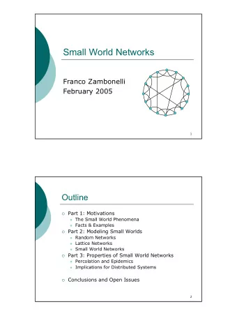
Small World Networks Dr. Natarajan Meghanathan Professor of Computer Science Jackson State University, Jackson, MS E-mail: natarajan.meghanathan@jsums.edu

Small-World Networks • A small-world network is a type of graph in which most nodes are not neighbors of one another, but most nodes can be reached from every other by a small number of hops. • Specifically, a small-world network is defined to be a network where the typical distance L (the number of hops) between two randomly chosen nodes grows proportionally to the logarithm of the number of nodes in the network. • Examples of Small-World Networks: – Road maps, food chains, electric power grids, metabolite processing networks, networks of brain neurons, voter networks, telephone call graphs, gene regulatory networks.

Small Worlds • Two major properties of small world networks – High average clustering coefficient • The neighbors of a node are connected to each other • Nodes’ contacts in a social network tend to know each other. – Short average shortest path length • Shorter paths between any two nodes in the network (Regular graph) (Small-world network) (Random graph) 0 Randomness 1

Triadic Closure and Growth Rate of New Friends Pure exponential growth No triadic closure Zero clustering coefficient Friends Friends of friends Triadic Closure reduces growth rate of new friends Increases clustering coefficient

Modeling Small World Networks • The ER model for random graphs provided shorter paths between any two nodes in the network. However, the ER graphs have a low clustering coefficient and triadic closures. – ER graphs have a constant, random and independent probability of two nodes being connected. • The Watts and Strogatz model (WS model) accounts for clustering while retaining the short average path lengths of the ER model. • The WS model interpolates between an ER graph and a regular ring lattice.

WS Model • Watts and Strogatz (WS) Model: The WS model interpolates between an ER graph and a regular ring lattice. – Let N be the number of nodes and K (assumed to be even) be the mean degree. – Assume N >> K >> ln(N) >> 1. – There is a rewiring parameter β (0 ≤ β ≤ 1). – Initially, let there be a regular ring lattice of N nodes, with K neighbors (K/2 neighbors on each side). – For every node n i = n 0 , n 1 , …, n N-1 , rewire the edge (n i , n j ), where i < j , with probability β . Rewiring is done by replacing (n i , n j ) with (n i , n k ) where n k is chosen uniform- randomly among all possible nodes that avoid self-looping and link duplication. β = 0 � � Regular ring lattice � � β = 1 � � � � Random network

Small-World Network: WS Model • The underlying lattice structure of the model produces a locally clustered network, and the random links dramatically reduce the average path lengths • The algorithm introduces about ( β NK/2) non-lattice edges. • Average Path Length ( β ): – Ring lattice L(0) = (N/2K) >> 1 – Random graph L(1) = (ln N / ln K) – For 0 < β < 1, the average path length reduces significantly even for smaller values of β . • Clustering Coefficient ( β ): − 3 ( K 2 ) K ( ) 3 = β = C − β C ( 0 ) C ' ( ) ( 0 ) * 1 = C ( 1 ) − 4 ( 1 ) K N – For 0 < β < 1, the clustering coefficient remains close to that of the regular lattice for low and moderate values of β and falls only at relatively high β . For low-moderate values of β , we thus capture the small-world • phenomenon where the average path length falls rapidly, while the clustering coefficient remains fairly high.

Limitations of the WS Model • The WS model introduced the notion of random edges to infuse shorter path lengths amidst larger clustering coefficient. • However, the long-range edges span between any two nodes in the network and do not mimic the edges of different lengths seen in real- world networks (like in the US road map as in Milgram’s experiment or airline map). – Path lengths could not be as small as they are in real networks. – Need some edges to nodes that are few hops away, rather than edges to some arbitrarily chosen nodes. – Cannot generate hubs as in scale-free networks. Source: Figure 20.4: Easley and Kleinberg

Enhancement to the WS Model • In addition to the re-wiring parameter β , another parameter called the clustering exponent (q) is introduced. • An (u, v) edge is selected for re-wiring with a probability β . After being selected, we do not randomly re-wire u with a node w. Instead, we pick a pair (u, w) for re-wiring with a probability of [d(u, w)- q ] / 2logn, where – For optimal results, q must be the dimensionality of the network modeled. For a ring lattice, q = 1. – n is the number of nodes in the network. – d(u, w) is the minimum number of hops between u and w in the original network layout (before enhancement) • The ring lattice is a single-dimension network • A grid is a two-dimensional network. – To implement this enhancement in simulations, we generate a random number between 0 to 1; the (u, w) pair whose [d(u, w)- dim ] / 2logn value is closest and above the random number generated is chosen for re-wiring. • With this re-wiring model, if routed optimally, (on average) the # hops in the path to the target is expected to reduce by a factor of 2 with every additional hop in the path [log n hops]