Slotted Aloha, instability D n is the drift , i.e. expected change in - PowerPoint PPT Presentation

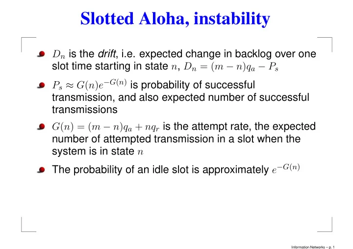
Slotted Aloha, instability D n is the drift , i.e. expected change in backlog over one slot time starting in state n , D n = ( m − n ) q a − P s P s ≈ G ( n ) e − G ( n ) is probability of successful transmission, and also expected number of successful transmissions G ( n ) = ( m − n ) q a + nq r is the attempt rate, the expected number of attempted transmission in a slot when the system is in state n The probability of an idle slot is approximately e − G ( n ) Information Networks – p. 1

Slotted Aloha, instability Departure/arrival rate as function of attempted rate for q r =0.2,0.3,0.4,0.6 0.4 0.35 0.3 0.25 0.2 0.15 0.1 0.05 0 0 2 4 6 8 10 12 Information Networks – p. 2

Slotted Aloha, instability Since G ( n ) e − G ( n ) is maximum 1 /e for G ( n ) = 1 we again see that maximum departure rate is 1 /e We can also see that they system may have two stable points and the departure rate is almost 0 at the other stable point, so if the system jumps to the undesirable stable point we can get departure rate almost 0 for a long time If we increase q r the delay in retransmitting collided packets decreases, but also the linear relationship between n and the attempt rate G ( n ) = mq a + n ( q r − q a ) changes ( G ( n ) increases with n faster when q r is increased) Information Networks – p. 3

Slotted Aloha, instability Increasing q r thus leads to fewer backlogged packets required to exceed the unstable equilibrium point Alternatively, if q r is decreased the delay increases and it becomes more difficult to exceed the unstable equilibrium point If q r is decreased enough only one stable point will remain, but then the backlog is a significant fraction of m so both an appreciable number of arriving packets are discarded and the delay is excessively large If we choose q r small enough for stable operation the delay is considerably greater than with TDM thus this approach is not of a very great practical importance Information Networks – p. 4

Slotted Aloha, instability If we replace the no-buffering assumption (a) with the infinite node assumption (b), the attempt rate becomes G ( n ) = λ + nq r , and the drift D n = λ − P s so the straight line in our graph becomes horizontal The undesirable stable point disappears, but once the system passes the unstable equilibrium it tends to increase without bound In this case there is no steady-state distribution for our infinite-state Markov model, and the expected backlog increases without bound From a practical point of view, if λ << 1 /e and q r is moderate then the system could be expected to remain in the desirable stable state for very long periods Information Networks – p. 5

Slotted Aloha, Stabilization Since P s = G ( n ) e − G ( n ) which is maximized when G ( n ) = 1 one approach to achieving stability is to change q r to maintain attempt rate G ( n ) at 1 The problem is that n is unknown to the nodes and can only be estimated from the feedback With no-buffering assumption (a) the system discards large numbers of arriving packages and has a very large but finite delay With infinite-node assumption (b) no arrivals are discarded but the delay becomes infinite We will now use the infinite-node assumption Information Networks – p. 6

Slotted Aloha, Stabilization We define a multiaccess system as stable for a given arrival rate if the expected delay per packet is finite The maximum stable throughput is defined as the least upper bound of arrival rates for which the system is stable The ordinary slotted Aloha has maximum stable throughput 0 When estimate of backlog is perfect and G ( n ) = 1 , idles occur with probability 1 /e ≈ 0 . 368 , success occur with probability 1 /e , and collisions occur with probability 1 − 2 /e ≈ 0 . 264 , thus the rule for changing q r should allow fewer collisions than idles Information Networks – p. 7

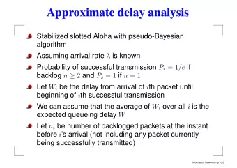
Slotted Aloha, Stabilization If all backlogged nodes use the same retransmission probability the maximum stable throughput is at most 1 /e , since when backlog is large the Poisson approximation becomes more accurate, the success rate is then limited to 1 /e and the drift is positive for λ > 1 /e Pseudo-Bayesian algorithm: new arrivals are regarded as backlogged immediately on arrival Attempt rate G ( n ) = nq r , probability of successful transmission is nq r (1 − q r ) n − 1 Each node maintains an estimate ˆ n of the backlog n at the beginning of each slot Information Networks – p. 8

Pseudo-Bayesian stabilization Each backlogged packed is transmitted with probability q r (ˆ n ) = min { 1 , 1 / ˆ n } The estimated backlog ˆ n k +1 at slot k + 1 is updated from the estimated backlog ˆ n k at slot k and feedback for slot k according to  max { λ, ˆ n k + λ − 1 } , for idle or success   n k +1 = ˆ n k + λ + ( e − 2) − 1 ,  ˆ for collision  Addition of λ to take new arrivals into account Subtraction of 1 for successful transmissions to account for succesful departure Information Networks – p. 9

Pseudo-Bayesian stabilization Subtracting of 1 for idle transmission for decreasing estimate when too many idle slots occur Adding ( e − 2) − 1 on collisions to increase estimate when too many collisions occur. For large backlogs, if ˆ n = n we get attempt rate 1, and idles with probability 1 /e , collision with probability ( e − 2) /e , so decreasing by 1 on idle and increasing by ( e − 2) − 1 on collision maintains balance between n and n on average ˆ Information Networks – p. 10

Pseudo-Bayesian stabilization Assume that probability distribution of n k is Poisson with mean ˆ n k ≥ 1 , i.e. n ν P ( n k = ν ) = ˆ ν ! e − ˆ k n k Each packet transmitted with probability 1 / ˆ n k n ν ∞ ∞ ˆ P ( n k = ν )(1 − 1 n k (1 − 1 ) ν = P ( idle ) � � ν ! e − ˆ k ) ν = n k ˆ n k ˆ ν =0 ν =0 n k − 1) ν ∞ (ˆ n k − 1 = e − 1 n k = e − ˆ � e − ˆ n k e ˆ = ν ! ν =0 Information Networks – p. 11

Pseudo-Bayesian stabilization The a posteriori probability that there were ν packets in the system given that the slot was idle is P ( idle | n k = ν ) P ( n k = ν ) P ( n k = ν | idle ) = P ( idle ) n ν n k ) ν · ˆ (1 − 1 ν ! e − ˆ n k n k − 1) ν k = (ˆ ˆ e − (ˆ n k − 1) = e − 1 ν ! Thus the a posteriori probability is Poisson distributed with mean ˆ n k − 1 Information Networks – p. 12

Pseudo-Bayesian stabilization Similarly the probability for successful transmission n ν ∞ ˆ n k ν (1 − 1 ) ν − 1 1 P ( succ ) � ν ! e − ˆ k = n k ˆ n k ˆ ν =0 ∞ n k − 1) ν − 1 (ˆ n k − 1 = e − 1 n k = e − ˆ � e − ˆ n k e ˆ = ( ν − 1)! ν =1 Information Networks – p. 13

Pseudo-Bayesian stabilization The a posteriori probability that there were ν + 1 packets in the system given that the slot had a successful transmission is P ( succ | n k = ν + 1) P ( n k = ν + 1) P ( n k = ν + 1 | succ ) = P ( succ ) n ν +1 ˆ ( ν + 1)(1 − 1 n k ) ν 1 ( ν +1)! e − ˆ n k n k · k ˆ ˆ = e − 1 n k − 1) ν (ˆ e − (ˆ n k − 1) = ν ! Thus the a posteriori probability for the remaining packets is Poisson distributed with mean ˆ n k − 1 Information Networks – p. 14

Pseudo-Bayesian stabilization Taking the new arrivals into account we get that given an a priori Poisson probability on n k with mean ˆ n k ≥ 1 , then given an idle or successful slot, the probability distribution of n k +1 is Poisson with mean n k + λ − 1 Given a collision, the a posteriori probability is not quite Poisson but may be reasonably approximated by a n k + λ + ( e − 2) − 1 Poisson with mean ˆ n k +1 = ˆ This is the reason the algorithm is called Pseudo-Bayesian Information Networks – p. 15

Pseudo-Bayesian stabilization In applications the arrival rate λ is typically unknown and slowly varying One possibility is to estimate λ by time-averaging rate of successful transmissions, however nothing has been proven about stability of the algorithm when using dynamic estimate of λ An alternative is to use a fixed value for λ , it can be shown that using 1 /e will give stability for all actual λ < 1 /e . Information Networks – p. 16

Markov chain example No-buffering assumption with m = 2 nodes, q a = 0 . 1 , q r = 0 . 3 . 0.01 0.03 0 1 2 0.99 0.58 0.27 0.42 0.7 The probabilities ( p ( k +1) , p ( k +1) , p ( k +1) ) for the states at slot 0 1 2 k + 1 can be expressed in the probabilities at slot k and the transition probabilities   0 . 99 0 0 . 01 ( p ( k +1) , p ( k +1) , p ( k +1) ) = ( p ( k ) 0 , p ( k ) 1 , p ( k ) 2 ) 0 . 27 0 . 7 0 . 03   0 1 2   0 0 . 42 0 . 58 Information Networks – p. 17

Markov chain example We thus have p ( k +1) = p ( k ) A = p ( k − 1) A 2 = . . . = p (0) A k +1 , where p (0) is the initial probability distribution at first time slot. Since the matrix has a right eigenvector (1 , 1 , 1) t with eigenvalue 1 , it also has a left eigenvector with eigenvalue 1. This is the largest possible eigenvalue and when k → ∞ the probability state will converge to this stationary probability distribution. The eigenvector equation system p ( A − I ) = 0 is underdetermined since it has a one-parameter solution space. By replacing one of the equations with the normalizing condition p 0 + p 1 + p 2 = 1 we get a unique solution. This means that we replace one of the columns with a column with only ones. Information Networks – p. 18