Single Source Shortest Paths (SSSP) Directed graph Edge weights - - PowerPoint PPT Presentation

Single Source Shortest Paths (SSSP)

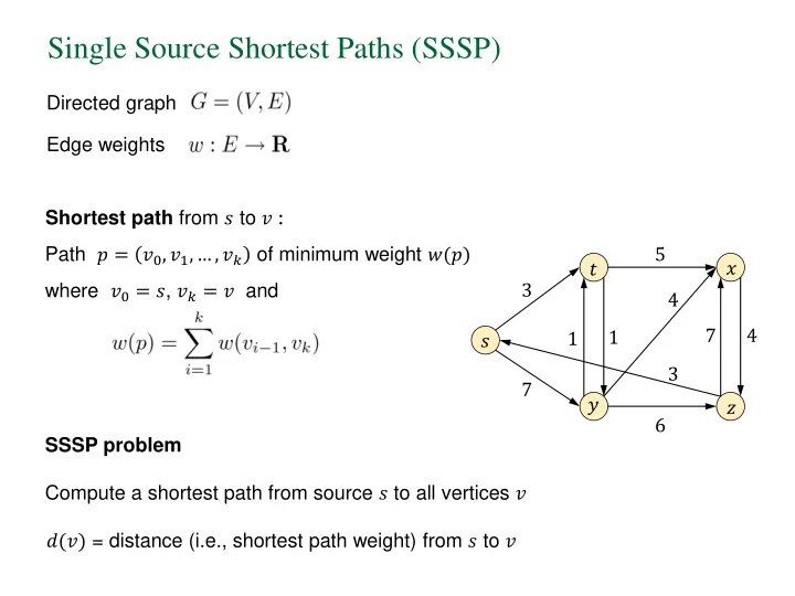
Edge weights Directed graph Path 𝑞 = 𝑤0, 𝑤1, … , 𝑤𝑙 of minimum weight 𝑥(𝑞) Shortest path from 𝑡 to 𝑤 : where 𝑤0 = 𝑡, 𝑤𝑙 = 𝑤 and SSSP problem Compute a shortest path from source 𝑡 to all vertices 𝑤 𝑢 𝑡 𝑦 𝑨 3 7 3 4 5 6 4 7 1 1 𝑒(𝑤) = distance (i.e., shortest path weight) from 𝑡 to 𝑤 𝑧

Single Source Shortest Paths (SSSP)

Edge weights Directed graph 𝑢 𝑡 𝑦 𝑨 3 7 3 4 5 6 4 7 1 1 Path 𝑞 = 𝑤0, 𝑤1, … , 𝑤𝑙 of minimum weight 𝑥(𝑞) Shortest path from 𝑡 to 𝑤 : where 𝑤0 = 𝑡, 𝑤𝑙 = 𝑤 and SSSP problem Compute a shortest path from source 𝑡 to all vertices 𝑤 𝑒(𝑢) = 3 𝑒(𝑧) = 4 𝑒(𝑦) = 8 𝑒(𝑧) = 10 𝑒(𝑤) = distance (i.e., shortest path weight) from 𝑡 to 𝑤 𝑧

Single Source Shortest Paths (SSSP)

Parent of a vertex Shortest paths tree Formed by the edges (𝑞(𝑤), 𝑤) 𝑞 𝑤 = vertex just before 𝑤 on the shortest path from 𝑡 𝑢 𝑡 𝑦 𝑨 3 7 3 4 5 6 4 7 1 1 𝑞(𝑤) 𝑡 𝑤 𝑞(𝑡) = - 𝑞(𝑢) = 𝑡 𝑞(𝑦) = 𝑢 𝑞(𝑧) = 𝑢 𝑞(𝑨) = 𝑧 𝑧

Single Source Shortest Paths (SSSP)

Temporary distances 𝑒(𝑤) = upper bound for the weight of the shortest path from 𝑡 to 𝑤 Initialize Edge relaxation 𝑞(𝑤) ← null, 𝑒(𝑤) ← ∞ for all 𝑤 ≠ 𝑡 𝑞(𝑡) ← null, 𝑒(𝑡) ← 0 relax(𝑣, 𝑤) if if 𝑒(𝑤) > 𝑒(𝑣) + 𝑥(𝑣, 𝑤) th then { 𝑒(𝑤) ← 𝑒(𝑣) + 𝑥(𝑣, 𝑤) 𝑞(𝑤) ← 𝑣 } 2 𝑒(𝑣) = 5 𝑣 𝑤 𝑒(𝑤) = 8 2 𝑒(𝑣) = 5 𝑣 𝑤 𝒆(𝒘) = 𝟖 2 𝑒(𝑣) = 5 𝑣 𝑤 𝑒(𝑤) = 6 2 𝑒(𝑣) = 5 𝑣 𝑤 𝑒(𝑤) = 6

Single Source Shortest Paths (SSSP)

Dijkstra’s Algorithm Used when edge weights are non-negative It maintains a set of vertices 𝑇 ⊆ 𝑊 for which a shortest path has been computed, i.e., the value of 𝑒(𝑤) is the exact weight of the shortest path to 𝑤. Each iteration selects a vertex 𝑣 ∈ 𝑊\S with minimum distance 𝑒(𝑣). Then we set S ← 𝑇 ∪ 𝑣 and relax all edges (𝑣, 𝑥) To find 𝑣 with min 𝑒(𝑣): Use a priority queue 𝑅 with keys

Single Source Shortest Paths (SSSP)

Dijkstra’s Algorithm Initialization 𝑞(𝑤) ← null, 𝑒(𝑤) ← ∞ for all 𝑤 ≠ 𝑡 𝑞(𝑡) ← null, 𝑒(𝑡) ← 0 insert all vertices 𝑤 into priority queue 𝑅 with key 𝑒(𝑤) set 𝑇 ← ∅ Main Loop while 𝑅 is not empty { 𝑣 ← Q. delMin() 𝑇 ← 𝑇 ∪ 𝑣 for all edges (𝑣, 𝑤) { relax(𝑣, 𝑤) } }

Single Source Shortest Paths (SSSP)

Dijkstra’s Algorithm Initialization 𝑞(𝑤) ← null, 𝑒(𝑤) ← ∞ for all 𝑤 ≠ 𝑡 𝑞(𝑡) ← null, 𝑒(𝑡) ← 0 insert all vertices 𝑤 into priority queue 𝑅 with key 𝑒(𝑤) set 𝑇 ← ∅ Main Loop while 𝑅 is not empty { 𝑣 ← Q. delMin() 𝑇 ← 𝑇 ∪ 𝑣 for all edges (𝑣, 𝑤) { relax(𝑣, 𝑤) } } priority queue 𝑅 running time array O(𝑜2) binary heap O(𝑛 log 𝑜) Fibonacci heap O(𝑛 + 𝑜 log 𝑜)

Single Source Shortest Paths (SSSP) in Map-Reduce

➢ Not easy to parallelize Dijkstra’s algorithm ➢ Use an iterative approach instead

• The distance 𝑒(𝑤) from 𝑡 to 𝑤 is updated by the distances of all 𝑣 with

𝑣, 𝑤 ∈ 𝐹.

• Need to communicate both distances and adjacency lists.

𝑧 𝑦 𝑤 𝑥(𝑦, 𝑤) 𝑨 𝑥(𝑧, 𝑤) 𝑥(𝑨, 𝑤) 𝑒(𝑤) ← min 𝑒 𝑣 + 𝑥 𝑣, 𝑤 | (𝑣, 𝑤) ∈ 𝐹

Single Source Shortest Paths (SSSP) in Map-Reduce

Mapper: emits distances and graph structure 𝑧 𝑦 𝑤 𝑥(𝑦, 𝑤) 𝑨 𝑥(𝑧, 𝑤) 𝑥(𝑨, 𝑤) 𝑒(𝑤) ← min 𝑒 𝑣 + 𝑥 𝑣, 𝑤 | (𝑣, 𝑤) ∈ 𝐹 Reducer: updates distances and emits graph structure 𝑏 𝑐 𝑤 𝑑 𝑒 𝑤 + 𝑥(𝑤, 𝑏) 𝑒 𝑤 + 𝑥(𝑤, 𝑐) 𝑒 𝑤 + 𝑥(𝑤, 𝑑)

Single Source Shortest Paths (SSSP) in Map-Reduce

➢ Not easy to parallelize Dijkstra’s algorithm ➢ Use an iterative approach instead

• The distance 𝑒(𝑤) from 𝑡 to 𝑤 is updated by the distances of all 𝑣 with

𝑣, 𝑤 ∈ 𝐹.

• Need to communicate both distances and adjacency lists.
• Repeat round until all distances are fixed.
• Number of rounds = 𝑜 − 1 in the worst case.
• If all weights are equal then we compute the Breadth-First Search

(BFS) tree. Number of rounds = graph diameter.

BFS in Map-Reduce

Single Source Shortest Paths (SSSP) in Map-Reduce

Remarks on Map-Reduce SSSP algorithm

• Essentially a brute-force algorithm.
• Performs many unnecessary computations.
• No global data structure.

PageRank in Map-Reduce

Recall the formula for the PageRank 𝑆(𝑣) of a webpage 𝑣

𝑆 𝑣 = 𝑑 ෍

𝑤∈𝐶𝑣

𝑆(𝑤) 𝑂𝑤 + (1 − 𝑑)𝐹𝑣

𝐶𝑣 = set of pages that point to 𝑣 𝐺

𝑣 = set of pages that 𝑣 points to

𝐺

𝑣 = 𝑂𝑣 = number of links from 𝑣

𝐹𝑣 = probabilities over web pages 𝐹𝑣 and 𝑑 are user designed parameters

PageRank in Map-Reduce

Iterative computation start with seed values 𝑆0(𝑤) for each page 𝑤 each page 𝑤 receives credit from the pages in 𝐶𝑤 and computes 𝑆𝑗+1(𝑤) each page 𝑤 distributes credit to the pages in 𝐺

𝑤

PageRank in Map-Reduce

Algorithms and Complexity in MapReduce (and related models)

Sorting, Searching, and Simulation in the MapReduce Framework

• M. T. Goodrich, N. Sitchinava, and Q. Zhang

ISAAC 2011 Fast Greedy Algorithms in MapReduce and Streaming

• R. Kumar, B. Moseley, S. Vassilvitskii, and A. Vattani

SPAA 2013 On the Computational Complexity of MapReduce

• B. Fish, J. Kun, A. D. Lelkes, L. Reyzin, and G. Turan

DISC 2015

• L. G. Valiant, A Bridging Model for Parallel Computation,

Communications of the ACM, 1990 Computational model of parallel computation BSP is a parallel programming model based on Synchronizer Automata. The model consists of:

• Set of processor-memory pairs.
• Communications network that delivers messages in a point-to-point

manner.

• Mechanism for the efficient barrier synchronization for all or a subset of

the processes.

• No special combining, replicating, or broadcasting facilities.

BSP model

• Vertical Structure

Supersteps: – Local computation – Process Communication – Barrier Synchronization

• Horizontal Structure

– Concurrency among a fixed number of virtual processors. – Processes do not have a particular order. – Locality plays no role in the placement of processes on processors.

Virtual Processors Local Computation Global Communication Barrier Synchronization

Implementation: BSPlib

BSP model

Simulation on MapReduce: 1. Create a tuple for each memory cell and processor. 2. Map each message to the destination processor label. 3. Reduce by performing one step of a processor, outputting the messages for next round. Theorem [Goodrich et al.]: Given a BSP algorithm 𝐵 that runs in 𝑈 supersteps with a total memory size 𝑂 using 𝑄 ≤ 𝑂 processors, we can simulate 𝐵 using O(𝑈) rounds and message complexity O(𝑈𝑂) in the memory-bound MapReduce framework with reducer memory size bounded by 𝑂/𝑄.

MapReduce simulation of a BSP program

Simulation on MapReduce: 1. Create a tuple for each memory cell and processor. 2. Map each message to the destination processor label. 3. Reduce by performing one step of a processor, outputting the messages for next round. Theorem [Goodrich et al.]: Given a BSP algorithm 𝐵 that runs in 𝑈 supersteps with a total memory size 𝑂 using 𝑄 ≤ 𝑂 processors, we can simulate 𝐵 using O(𝑈) rounds and message complexity O(𝑈𝑂) in the memory-bound MapReduce framework with reducer memory size bounded by 𝑂/𝑄. A corollary of the above: Given the optimal BSP algorithm of [Goodrich, 99], we can sort 𝑂 values in the MapReduce framework in 𝑃(𝑙) rounds and 𝑃(𝑙𝑂) message complexity.

MapReduce simulation of a BSP program

Algorithms and Complexity in MapReduce (and related models)

Theorem [Fish et al.] : Any problem requiring sublogarithmic space, 𝑝(log 𝑜 ), can be solved in MapReduce in two rounds. The proof is constructive: Given a problem that classically takes less than logarithmic space, there is an automatic algorithm to implement it in MapReduce