Single-cell RNA-sequencing Ximena Ibarra-Soria CRUK Cambridge - PowerPoint PPT Presentation
Single-cell RNA-sequencing Ximena Ibarra-Soria CRUK Cambridge Institute RNA-Sequence Analysis Course - EMBL EBI 12 April 2019 Based on materials by Aaron Lun Why use single-cell RNA-seq It allows us to chracterise heterogeneity in the gene
Single-cell RNA-sequencing Ximena Ibarra-Soria CRUK Cambridge Institute RNA-Sequence Analysis Course - EMBL EBI 12 April 2019 Based on materials by Aaron Lun
Why use single-cell RNA-seq It allows us to chracterise heterogeneity in the gene expression profile of a population. The cell is the basic unit of life. At the cell-level we can:
Why use single-cell RNA-seq It allows us to chracterise heterogeneity in the gene expression profile of a population. The cell is the basic unit of life. At the cell-level we can: ◮ Define cell identities (e.g. cell-types or subtypes). doi.org/10.1038/nri2707 doi.org/10.15252/msb.20145549
Why use single-cell RNA-seq It allows us to chracterise heterogeneity in the gene expression profile of a population. The cell is the basic unit of life. At the cell-level we can: ◮ Define cell identities (e.g. cell-types or subtypes). ◮ Observe cell states and behaviour (e.g. cell cycle, metabolism, stress). doi.org/10.1038/nri2707 doi.org/10.15252/msb.20145549
Why use single-cell RNA-seq It allows us to chracterise heterogeneity in the gene expression profile of a population. The cell is the basic unit of life. At the cell-level we can: ◮ Define cell identities (e.g. cell-types or subtypes). ◮ Observe cell states and behaviour (e.g. cell cycle, metabolism, stress). ◮ Study dynamic processes (e.g. differentiation, activation). doi.org/10.1038/nri2707 doi.org/10.15252/msb.20145549
Why use single-cell RNA-seq It allows us to chracterise heterogeneity in the gene expression profile of a population. The cell is the basic unit of life. At the cell-level we can: ◮ Define cell identities (e.g. cell-types or subtypes). ◮ Observe cell states and behaviour (e.g. cell cycle, metabolism, stress). ◮ Study dynamic processes (e.g. differentiation, activation). ◮ Study noise in transcriptional regulation. doi.org/10.1038/nri2707 doi.org/10.15252/msb.20145549
Why use single-cell RNA-seq RNA-seq allows quantification of the whole transcriptome. ◮ FISH: small number of transcripts. ◮ seqFISH+: 10,000 genes. ◮ FACS: small number of proteins. ◮ Mass cytometry: ~40 proteins.
A typical single-cell experiment Tissue Dissociated Physical separation Lysis single cells ACTG CCTG GCTA 3'-TTTTTTTTT-X-5' T A C AAAAAAAA G T G T G C C A C Computational ACTG GCTA CCTG G T ACTG GCTA C A CCTG C T G C analysis G T C A Pooled sequencing Cell barcoding Reverse transcription ◮ Dissociation can be easy or hard (blood vs muscle). ◮ Many separation methods (plate-based, droplets). ◮ Different protocols for RT and cDNA generation (full-length, 5’/3’ biased)
Throughput of scRNA-seq protocols scRNA-seq protocols have increased hugely in throughput. ◮ Cell separation using FACS or microfluidic devices. ◮ Automation of RT and cDNA generation. a Manual Multiplexing Integrated fluidic Liquid-handling Nanodroplets Picowells In situ barcoding circuits robotics Tang et al. 2009 18 Islam et al. 2011 24 Brennecke et al. 2013 64 Jaitin et al. 2014 33 Klein et al. 2015 34 Bose et al. 2015 43 Cao et al. 2017 51 Macosko et al. 2015 40 Rosenberg et al. 2017 52 b 10x Genomics SPLiT-seq 1,000,000 Drop-seq sci-RNA-seq 100,000 MARS-seq CytoSeq inDrop Single cells in study DroNC-seq 10,000 Seq-Well High-throughput STRT-seq CEL-seq Fluidigm C1 1,000 sequencing of RNA from single cells 100 10 SMART-seq2 SMART-seq 1 2009 2010 2011 2012 2013 2014 2015 2016 2017 Study publication date Svensson et al. , Nature Protocols, 2018 (doi.org/10.1038/nprot.2017.149)
scRNA-seq protocols Plate-based Droplet-based ◮ Hundreds to a few ◮ Tens to hundreds of thousand cells. thousands cells. ◮ High number of genes ◮ Lower number of genes detected. detected. ◮ High capture efficiency. ◮ Variable capture efficiency. ◮ Full-length transcripts. ◮ 3’/5’-biased. ◮ UMIs optional. ◮ UMIs. ◮ Compatible with spike-ins. ◮ No spike-ins.
Library prep ◮ Most protocols use polyA selection. ◮ cDNA is amplified by PCR. ◮ Introduction of strong biases. ◮ Alleviated by the use of U nique M olecular I dentifiers (UMIs). After RT After amplification Transcript (RC) 3'-ACATCGATCGC...TTTT-GGAT-AACGT-5' Constant 3'-ACATCGATCGC...TTTT-GGAT-AACGT-5' 3'-ACATCGATCGC...TTTT-GGAT-AACGT-5' 3'-ACATCGATCGC...TTTT-GGAT-AACGT-5' 3'-ACATCGATCGC...TTTT-GGAT-AACGT-5' 3'-ACATCGATCGC...TTTT-GGAT-AACGT-5' UMI 3'-CGACGGTTACG...TTTT-GCTT-AACGT-5' 3'-CGACGGTTACG...TTTT-GCTT-AACGT-5' 3'-TGAGCATCACTA...TTTT-AGTA-AACGT-5' 3'-TGAGCATCACTA...TTTT-AGTA-AACGT-5' 3'-TGAGCATCACTA...TTTT-AGTA-AACGT-5' 3'-TGAGCATCACTA...TTTT-AGTA-AACGT-5' After fragmentation After sequencing 3'-CAGTCGTACG...TTTT-GGAT-AACGT-5' Read 2 Read 1 3'-CGAGGGCGGT...TTTT-GGAT-AACGT-5' GTCAGCATGC TAGG 3'-AGCGTAGGCT...TTTT-GGAT-AACGT-5' GCTCCCGCCA TAGG 3'-CAGGCTGACG...TTTT-GGAT-AACGT-5' TCGCATCCGA TAGG 3'-GGATAGCTAG...TTTT-GGAT-AACGT-5' GACCGACTGC TAGG CCTATCGATC TAGG 3'-CACGGAAAAT...TTTT-GCTT-AACGT-5' GAGCCTTTTA TTCG GTCGTCGACT ATGA 3'-CAGCAGCTGA...TTTT-AGTA-AACGT-5' GGCCCCTCCT ATGA 3'-CCGGGGAGGA...TTTT-AGTA-AACGT-5' GAAAATACTC ATGA 3'-CTTTTATGAG...TTTT-AGTA-AACGT-5' Different fragmentation site per amplicon
Cell barcoding Allows multiplexing to sequence many libraries in the same lane. Different strategies: 1. Cell barcode in the PCR primer. ◮ Incorporated during library prep. ◮ Plate-based methods only (different barcode per well). 2. Cell barcode in the oligo-dT primer. Cell barcode (constant within bead) Bead CGACTA-NNNN-TTTTTTTT-3' UMI (variable within bead) Di fferent cell barcode Bead GTCAAA-NNNN-TTTTTTTT-3' One bead loaded per droplet, as well as ≤ 1 cell (hopefully)
scRNA-seq data In its rawest form, FASTQ files after Illumina sequencing. 1. Align reads to reference genome. ◮ Many good and fast aligners (e.g. subread, STAR). 2. Count number of reads mapped to each gene (e.g. HTSeq, featureCounts). This produces a count matrix with one count per gene per cell.
scRNA-seq data In its rawest form, FASTQ files after Illumina sequencing. 1. Align reads to reference genome. ◮ Many good and fast aligners (e.g. subread, STAR). 2. Count number of reads mapped to each gene (e.g. HTSeq, featureCounts). This produces a count matrix with one count per gene per cell. ◮ If UMIs are used, reads with the same UMI are collapsed to a single count.
scRNA-seq data In its rawest form, FASTQ files after Illumina sequencing. 1. Align reads to reference genome. ◮ Many good and fast aligners (e.g. subread, STAR). 2. Count number of reads mapped to each gene (e.g. HTSeq, featureCounts). This produces a count matrix with one count per gene per cell. ◮ If UMIs are used, reads with the same UMI are collapsed to a single count. ◮ Data generated with the 10X platform can be processed with CellRanger .
scRNA-seq data A typical scRNA-seq data count matrix ◮ Lots of zeros (both dropouts and lack of expression). ~100 - 1000 cells ~10000-40000 genes
scRNA-seq data ◮ Lots of zeros (both dropouts and lack of expression). 5000 pg 500 pg a b 10 7 10 7 (5,000 pg, technical replicate 2 ) (500 pg, technical replicate 2 ) 10 5 10 5 Normalized read count Normalized read count 10 3 10 3 10 10 0 0 10 3 10 5 10 7 10 3 10 5 10 7 0 10 0 10 Normalized read count Normalized read count (5,000 pg, technical replicate 1 ) (500 pg, technical replicate 1 ) 50 pg 10 pg c d 10 7 10 7 (50 pg, technical replicate 2 ) (10 pg, technical replicate 2 ) 10 5 10 5 Normalized read count Normalized read count 10 3 10 3 10 10 0 0 10 3 10 5 10 7 10 3 10 5 10 7 0 10 0 10 Normalized read count Normalized read count (50 pg, technical replicate 1 ) (10 pg, technical replicate 1 ) Brennecke et al., Nat Methods, 2013
scRNA-seq data analysis Aim : to extract real biology from data with technical noise 1. Quality control. 2. Normalisation of cell-specific biases. 3. Batch correction. 4. Modelling technical noise. 5. Dimensionality reduction and visualisation. 6. Clustering. . . . followed by higher-level analyses and interpretation.
Quality control Removal of low-quality cells arising by: ◮ Insufficient sequencing. ◮ Failed reverse transcription. ◮ Damaged cells during dissociation.
Quality control We use several metrics to identify low-quality samples: ◮ Total number of reads per cell ( low ). ◮ Total number of genes detected ( low ). ◮ Percentage of reads mapped to mitochondrial genes ( high ). ◮ Percentage of reads mapped to spike-in transcripts ( high ). Coverage Coverage Coverage Damage Non-mito Non-mito Non-mito Mito Mito Mito Extreme damage Spike-in Spike-in Spike-in
Quality control QC metrics. 7 15000 6 total_features_by_counts log10_total_counts 10000 5 5000 4 3 0 2383 2384 2677 2739 2383 2384 2677 2739 sample sample Data from Messmer et al., Cell Reports (2019).
Quality control QC metrics. 100 20 75 15 pct_counts_ERCC pct_counts_Mt 50 10 25 5 0 0 2383 2384 2677 2739 2383 2384 2677 2739 sample sample Data from Messmer et al., Cell Reports (2019).
Quality control How to define low-quality ? 1. Define fixed thresholds, e.g., at least 100,000 counts per cell. ◮ simple, easy to interpret. ◮ hard to generalize across data sets.
Recommend
More recommend
Explore More Topics
Stay informed with curated content and fresh updates.

