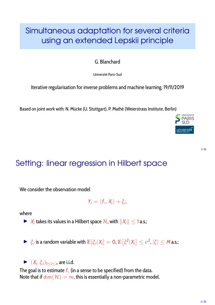
Simultaneous adaptation for several criteria using an extended - PDF document

Simultaneous adaptation for several criteria using an extended Lepskii principle G. Blanchard Université Paris-Sud Iterative regularisation for inverse problems and machine learning, 19/11/2019 Based on joint work with: N. Mücke (U. Stuttgart), P. Mathé (Weierstrass Institute, Berlin) 1 / 25 Setting: linear regression in Hilbert space We consider the observation model Y i = � f ◦ , X i � + ξ i , where ◮ X i takes its values in a Hilbert space H , with � X i � ≤ 1 a.s.; � ≤ σ 2 , | ξ | ≤ M a.s.; � ξ 2 | X i ◮ ξ i is a random variable with E [ ξ i | X i ] = 0, E ◮ ( X i , ξ i ) 1 ≤ i ≤ n are i.i.d. The goal is to estimate f ◦ (in a sense to be specified) from the data. Note that if dim ( H ) = ∞ , this is essentially a non-parametric model. 2 / 25

Why this model? ◮ Hilbert-space valued variables appear in standard models of Functional Data Analysis , where the observed data are modeled (idealized) as function-valued. ◮ Such models also appear in reproducing kernel Hilbert space (RKHS) methods in machine learning: ◮ assume observations X i take valued in some space X ◮ let Φ : X → H be a “feature mapping” in a Hilbert space H , and � X = Φ ( X ) , then one considers the model � + ξ i = � � f ◦ , � Y i = f ◦ ( X i ) + ξ i , X i where � f ∈ � H : = { x �→ � f , Φ ( x ) � ; f ∈ H} is a nonparametric model of functions (nonlinear in x !). ◮ Usually all computations don’t require explicit knowledge of Φ but only access to the kernel k ( x , x ′ ) = � Φ ( x ) , Φ ( x ′ ) � . 3 / 25 Why this model (II) - inverse learning Of interest is also the inverse learning problem: ◮ X i takes value in X ; ◮ if A is a linear operator from a Hilbert space H to a real function space on X ; ◮ inverse regression learning model: Y i = ( Af ◦ )( X i ) + ξ i . ◮ If A is a Carleman operator (i.e. evaluation functionals f �→ ( Af )( x ) are continuous for all x ), then this can be isometrically reduced to a reproducing kernel learning setting (De Vito, Rosasco, Caponnetto 2006; Blanchard and Mücke, 2017). 4 / 25

Two notions of risk We will consider two notions of error (risk) for a candidate estimate � f of f ◦ : ◮ Squared prediction error: ���� � 2 � � − Y E ( � f ) : = E f , X . ◮ The associated (excess error) risk is ��� �� 2 � � � 2 � � f ∗ − f ∗ E ( � � �� f ) − E ( f ◦ ) = E f − f ◦ , X = � 2 , X , ◦ ◮ Reconstruction error risk: � � 2 � � �� f − f ◦ � H . The goal is to find a suitable estimator � f of f ◦ from the data having “optimal” convergence properties with respect to these two risks. 5 / 25 Finite-dimensional case ◮ The final dimensional case: X = R p , f ◦ now denoted β ◦ ◮ In usual matrix form: Y = X β ◦ + ξ . ◮ X T i form the lines of the ( n , p ) design matrix X ◮ Y = ( Y 1 , . . . , Y n ) T ◮ ξ = ( ξ 1 , . . . , ξ n ) T � � � 2 . � β ◦ − � ◮ “Reconstruction” risk corresponds to β ◮ Prediction risk corresponds to �� � 2 � � � � 2 , β ◦ − � � Σ 1 / 2 ( β ◦ − � β , X = β ) E � XX T � where Σ : = E . ◮ In Hilbert space, same relation with Σ : = E [ X ⊗ X ∗ ] . 6 / 25

The founding fathers of machine learning? A.M. Legendre C.F. Gauß The “ordinary” least squares (OLS) solution: β OLS = ( X T X ) − 1 X T Y . � 7 / 25 Convergence of OLS in finite dimension ◮ We want to understand the behavior of � β OLS , when the data size n grows large. Will we be close to the truth β ◦ ? ◮ Recall � � − 1 � 1 � − 1 � 1 � X T X X T Y = n X T X n X T Y � = � Σ − 1 � β OLS = γ , � �� � � �� � : = � : = � γ Σ ◮ Observe by a vectorial LLN, as n → ∞ : � � n Σ : = 1 n X T X = 1 � X i X T X 1 X T ∑ − → E = : Σ ; i 1 n ���� i = 1 = : Z ′ i n γ : = 1 n X T Y = 1 ∑ � − → E [ X 1 Y 1 ] = Σ β ◦ = : γ ; X i Y i ���� n i = 1 = : Z i ◮ Hence � β = � Σ − 1 � γ → Σ − 1 γ = β ◦ . (Assuming Σ invertible.) 8 / 25

From OLS to Hilbert-space regression ◮ For ordinary linear regression with X = R p (fixed p , n → ∞ ): ◮ LLN implies � β OLS (= � Σ − 1 � γ ) → β ◦ (= Σ − 1 γ ) ; ◮ CLT+Delta Method imply asymptotic normality and convergence in O ( n − 1 2 ) . ◮ How to generalize to X = H ? ◮ Main issue: Σ = E [ X ⊗ X ∗ ] does not have a continuous inverse. ( → ill-posed problem) Σ ) of Σ − 1 (regularization) , where ◮ Need to consider a suitable approximation ζ ( � m Σ : = 1 � X i ⊗ X ∗ ∑ i n i = 1 is the empirical second moment operator. 9 / 25 Regularization methods Σ − 1 by an approximate inverse, such as ◮ Main idea: replace � ◮ Ridge regression/Tikhonov : � f Ridge ( λ ) = ( � Σ + λ I p ) − 1 � γ ◮ PCA projection/spectral cut-off : restrict � Σ on its k first eigenvectors � f PCA ( k ) = ( � Σ ) − 1 | k � γ ◮ Gradient descent/Landweber Iteration/ L 2 boosting : � f LW ( k ) = � Σ � γ − � f LW ( k − 1 ) + ( � f LW ( k − 1 ) ) k Σ ) k � ( I − � ∑ = γ , i = 0 � � �� � Σ op ≤ 1). (assuming 10 / 25

General form spectral linearization Bauer, Rosasco, Pereverzev 2007 ◮ General form regularization method: � f λ = ζ λ ( � Σ ) � γ for some well-chosen function ζ λ : R + → R + acting on the spectrum and “approximating” the function x �→ x − 1 . ◮ λ > 0: regularization parameter; λ → 0 ⇔ less regularization ◮ Notation of (autoadjoint) functional calculus, i.e. Σ = Q T diag ( µ 1 , µ 2 , . . . ) Q ⇒ ζ ( � Σ ) : = Q T diag ( ζ ( µ 1 ) , ζ ( µ 2 ) , . . . ) Q � ◮ Examples (revisited): ◮ Tikhonov : ζ λ ( t ) = ( t + λ ) − 1 ◮ Spectral cut-off : ζ λ ( t ) = t − 1 1 { t ≥ λ } i = 0 ( 1 − t ) i . ◮ Landweber iteration : ζ k ( t ) = ∑ k 11 / 25 Assumptions on regularization function Standard assumptions on the regularization family ζ λ : [ 0 , 1 ] → R are: (i) There exists a constant D < ∞ such that | t ζ λ ( t ) | ≤ D , sup sup 0 < λ ≤ 1 0 < t ≤ 1 (ii) There exists a constant E < ∞ such that λ | ζ λ ( t ) | ≤ E , sup sup 0 < λ ≤ 1 0 < t ≤ 1 (iii) Qualification: for residual r λ ( t ) : = 1 − t ζ λ ( t ) , | r λ ( t ) | t ν ≤ γ ν λ ν , ∀ λ ≤ 1 : sup 0 < t ≤ 1 holds for ν = 0 and ν = q > 0. 12 / 25

Structural Assumptions (I) ◮ Denote ( µ i ) i ≥ 1 the sequence of positive eigenvalues of Σ in nonincreasing order. ◮ Assumptions on spectrum decay: for s ∈ ( 0 , 1 ) ; α > 0: µ i ≤ α i − 1 IP < ( s , α ) : s ◮ This implies quantitative estimates of the “effective dimension” N ( λ ) : = Tr ( ( Σ + λ ) − 1 Σ ) � λ − s . 13 / 25 Structural Assumptions (II) ◮ Denote ( µ i ) i ≥ 1 the sequence of positive eigenvalues of Σ in nonincreasing order. ◮ Source condition for the signal: for r > 0, define f ◦ = Σ r h ◦ for some h ◦ with � h ◦ � ≤ R , SC ( r , R ) : or equivalently, as a Sobolev-type regularity � � f ∈ H : ∑ µ − 2 r f 2 i ≤ R 2 SC ( r , R ) : f ◦ ∈ , i i ≥ 1 where f i are the coefficients of h in the eigenbasis of Σ . ◮ Under ( SC )( r , R ) it is assumed that the qualification q of the regularization method satisfies q ≥ r + 1 2 . 14 / 25

A general upper bound risk estimate Theorem Assume the source condition ( SC )( r , R ) holds. If λ is such that λ � ( N ( λ ) ∨ log ( η ) 2 ) / n, then with probability at least 1 − η , it holds: � ( Σ + λ ) 1 / 2 � � �� � � f ◦ − � f λ � H � � � N ( λ ) 1 R λ r + 1 + O ( n − 1 � log ( η ) 2 2 + σ 2 ) √ + . n n λ This gives rise to estimates in both norms of interest since � � � �� � ( Σ + λ ) 1 / 2 � � � � � H ≤ λ − 1 � f ◦ − � f ◦ − � f λ � f λ � H , 2 and � � � � � ( Σ + λ ) 1 / 2 � � �� � � � � � � 1 � f ∗ ◦ − � f ∗ 2 ( f ◦ − � f ◦ − � L 2 ( P X ) = � Σ f λ ) H ≤ f λ � � � H . λ 15 / 25 Upper bound on rates Optimizing the obtained bound over λ (i.e. balancing the main terms) one obtains Theorem Assume r , R , s , α are fixed positive constants and assume P XY satisfies (IP < ) ( s , α ) , (SC) ( r , R ) and � X � ≤ 1 , � Y � ≤ M, Var [ Y | X ] ∞ ≤ σ 2 a.s. Define � β n = ζ λ n ( � Σ ) � γ , using a regularization family ( ζ λ ) satisfying the standard assumptions with qualification q ≥ r + 1 2 , and the parameter choice rule � � − 1 R 2 σ 2 / n 2 r + 1 + s . λ n = Then it holds for any p ≥ 1 : n → ∞ E ⊗ n �� � p � 1 / p � � σ 2 � r 2 r + 1 + s ≤ C � ; � � � f ◦ − � f λ n � R lim sup R 2 n n → ∞ E ⊗ n �� � � 1 / p � � σ 2 � r + 1 / 2 p 2 r + 1 + s ≤ C � . � � � f ∗ ◦ − � f λ n R lim sup � R 2 n 2 , X 16 / 25