Simple mechanisms for escaping from local optima: I Restart: - PDF document

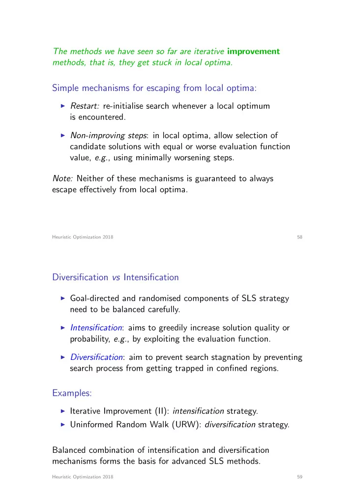
The methods we have seen so far are iterative improvement methods, that is, they get stuck in local optima. Simple mechanisms for escaping from local optima: I Restart: re-initialise search whenever a local optimum is encountered. I Non-improving steps : in local optima, allow selection of candidate solutions with equal or worse evaluation function value, e.g. , using minimally worsening steps. Note: Neither of these mechanisms is guaranteed to always escape e ff ectively from local optima. Heuristic Optimization 2018 58 Diversification vs Intensification I Goal-directed and randomised components of SLS strategy need to be balanced carefully. I Intensification : aims to greedily increase solution quality or probability, e.g. , by exploiting the evaluation function. I Diversification : aim to prevent search stagnation by preventing search process from getting trapped in confined regions. Examples: I Iterative Improvement (II): intensification strategy. I Uninformed Random Walk (URW): diversification strategy. Balanced combination of intensification and diversification mechanisms forms the basis for advanced SLS methods. Heuristic Optimization 2018 59

‘Simple’ SLS Methods Goal: E ff ectively escape from local minima of given evaluation function. General approach: For fixed neighbourhood, use step function that permits worsening search steps . Specific methods: I Randomised Iterative Improvement I Probabilistic Iterative Improvement I Simulated Annealing I Tabu Search I Dynamic Local Search Heuristic Optimization 2018 60 Randomised Iterative Improvement Key idea: In each search step, with a fixed probability perform an uninformed random walk step instead of an iterative improvement step. Randomised Iterative Improvement (RII): determine initial candidate solution s While termination condition is not satisfied: | | With probability wp : choose a neighbour s 0 of s uniformly at random | | | | Otherwise: choose a neighbour s 0 of s such that g ( s 0 ) < g ( s ) or, | | if no such s 0 exists, choose s 0 such that g ( s 0 ) is minimal | | b s := s 0 Heuristic Optimization 2018 61

Note: I No need to terminate search when local minimum is encountered Instead: Bound number of search steps or CPU time from beginning of search or after last improvement. I Probabilistic mechanism permits arbitrary long sequences of random walk steps Therefore: When run su ffi ciently long, RII is guaranteed to find (optimal) solution to any problem instance with arbitrarily high probability. I A variant of RII has successfully been applied to SAT (GWSAT algorithm), but generally, RII is often outperformed by more complex SLS methods. Heuristic Optimization 2018 62 Example: Randomised Iterative Best Improvement for SAT procedure GUWSAT ( F , wp , maxSteps ) input: propositional formula F , probability wp , integer maxSteps output: model of F or ∅ choose assignment a of truth values to all variables in F uniformly at random; steps := 0; while not ( a satisfies F ) and ( steps < maxSteps ) do with probability wp do select x uniformly at random from set of all variables in F ; otherwise select x uniformly at random from { x 0 | x 0 is a variable in F and changing value of x 0 in a max. decreases number of unsat. clauses } ; change value of x in a ; steps := steps +1; end if a satisfies F then return a else return ∅ end end GUWSAT Heuristic Optimization 2018 63

Note: I A variant of GUWSAT, GWSAT [Selman et al., 1994], was at some point state-of-the-art for SAT I Generally, RII is often outperformed by more complex SLS methods I Very easy to implement I Very few parameters Heuristic Optimization 2018 64 Probabilistic Iterative Improvement Key idea: Accept worsening steps with probability that depends on respective deterioration in evaluation function value: bigger deterioration ⇠ = smaller probability Realisation : I Function p ( g , s ): determines probability distribution over neighbours of s based on their values under evaluation function g . I Let step ( s )( s 0 ) := p ( g , s )( s 0 ). Note : I Behaviour of PII crucially depends on choice of p . I II and RII are special cases of PII. Heuristic Optimization 2018 65

Example: Metropolis PII for the TSP (1) I Search space: set of all Hamiltonian cycles in given graph G . I Solution set: same as search space ( i.e. , all candidate solutions are considered feasible). I Neighbourhood relation: reflexive variant of 2-exchange neighbourhood relation (includes s in N ( s ), i.e. , allows for steps that do not change search position). Heuristic Optimization 2018 66 Example: Metropolis PII for the TSP (2) I Initialisation: pick Hamiltonian cycle uniformly at random. I Step function: implemented as 2-stage process: 1. select neighbour s 0 2 N ( s ) uniformly at random; 2. accept as new search position with probability: 1 if f ( s 0 )  f ( s )   p ( T , s , s 0 ) := exp( f ( s ) � f ( s 0 ) ) otherwise  T ( Metropolis condition ), where temperature parameter T controls likelihood of accepting worsening steps. I Termination: upon exceeding given bound on run-time. Heuristic Optimization 2018 67

Simulated Annealing Key idea: Vary temperature parameter, i.e. , probability of accepting worsening moves, in Probabilistic Iterative Improvement according to annealing schedule (aka cooling schedule ). Inspired by a simulation of the physical annealing process: I candidate solutions ⇠ = states of physical system I evaluation function ⇠ = thermodynamic energy I globally optimal solutions ⇠ = ground states I parameter T ⇠ = physical temperature Note: In physical process ( e.g. , annealing of metals), perfect ground states are achieved by very slow lowering of temperature. Heuristic Optimization 2018 68 Simulated Annealing (SA): determine initial candidate solution s set initial temperature T according to annealing schedule While termination condition is not satisfied: | probabilistically choose a neighbour s 0 of s | | using proposal mechanism | | If s 0 satisfies probabilistic acceptance criterion (depending on T ): | | s := s 0 | b update T according to annealing schedule Heuristic Optimization 2018 69

Note: I 2-stage step function based on I proposal mechanism (often uniform random choice from N ( s )) I acceptance criterion (often Metropolis condition ) I Annealing schedule (function mapping run-time t onto temperature T ( t )): I initial temperature T 0 (may depend on properties of given problem instance) I temperature update scheme ( e.g. , geometric cooling: T := α · T ) I number of search steps to be performed at each temperature (often multiple of neighbourhood size) I Termination predicate: often based on acceptance ratio , i.e. , ratio of proposed vs accepted steps. Heuristic Optimization 2018 70 Example: Simulated Annealing for the TSP Extension of previous PII algorithm for the TSP, with I proposal mechanism: uniform random choice from 2-exchange neighbourhood; I acceptance criterion: Metropolis condition (always accept improving steps, accept worsening steps with probability exp [( f ( s ) � f ( s 0 )) / T ]); I annealing schedule : geometric cooling T := 0 . 95 · T with n · ( n � 1) steps at each temperature ( n = number of vertices in given graph), T 0 chosen such that 97% of proposed steps are accepted; I termination: when for five successive temperature values no improvement in solution quality and acceptance ratio < 2%. Heuristic Optimization 2018 71

Improvements: I neighbourhood pruning ( e.g. , candidate lists for TSP) I greedy initialisation ( e.g. , by using NNH for the TSP) I low temperature starts (to prevent good initial candidate solutions from being too easily destroyed by worsening steps) I look-up tables for acceptance probabilities: instead of computing exponential function exp( ∆ / T ) for each step with ∆ := f ( s ) � f ( s 0 ) (expensive!), use precomputed table for range of argument values ∆ / T . Heuristic Optimization 2018 72 Example: Simulated Annealing for the graph bipartitioning I for a given graph G := ( V , E ), find a partition of the nodes in two sets V 1 and V 2 such that | V 1 | = | V 2 | , V 1 [ V 2 = V , and that the number of edges with vertices in each of the two sets is minimal B A Heuristic Optimization 2018 73

SA example: graph bipartitioning Johnson et al. 1989 I tests were run on random graphs ( G n , p ) and random geometric graphs U n , d I modified cost function ( α : imbalance factor) f ( V 1 , V 2 ) = |{ ( u , v ) 2 E | u 2 V 1 ^ v 2 V 2 }| + α ( | V 1 | � | V 2 | ) 2 allows infeasible solutions but punishes the amount of infeasibility I side advantage : allows to use 1–exchange neighborhoods of size O ( n ) instead of the typical neighborhood that exchanges two nodes at a time and is of size O ( n 2 ) Heuristic Optimization 2018 74 SA example: graph bipartitioning Johnson et al. 1989 I initial solution is chosen randomly I standard geometric cooling schedule I experimental comparison to Kernighan–Lin heuristic I Simulated Annealing gave better performance on G n , p graphs I just the opposite is true for U n , d graphs I several further improvements were proposed and tested general remark: Although relatively old, Johnson et al.’s experimental investigations on SA are still worth a detailed reading! Heuristic Optimization 2018 75