Similarity Metrics and Efficient Optimization for Simultaneous - PDF document

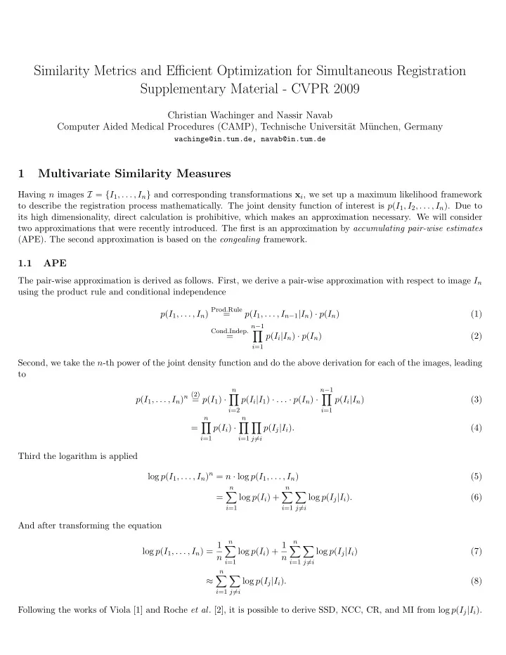
Similarity Metrics and Efficient Optimization for Simultaneous Registration Supplementary Material - CVPR 2009 Christian Wachinger and Nassir Navab Computer Aided Medical Procedures (CAMP), Technische Universit¨ at M¨ unchen, Germany wachinge@in.tum.de, navab@in.tum.de 1 Multivariate Similarity Measures Having n images I = { I 1 , . . . , I n } and corresponding transformations x i , we set up a maximum likelihood framework to describe the registration process mathematically. The joint density function of interest is p ( I 1 , I 2 , . . . , I n ). Due to its high dimensionality, direct calculation is prohibitive, which makes an approximation necessary. We will consider two approximations that were recently introduced. The first is an approximation by accumulating pair-wise estimates (APE). The second approximation is based on the congealing framework. 1.1 APE The pair-wise approximation is derived as follows. First, we derive a pair-wise approximation with respect to image I n using the product rule and conditional independence p ( I 1 , . . . , I n ) Prod.Rule = p ( I 1 , . . . , I n − 1 | I n ) · p ( I n ) (1) n − 1 Cond.Indep. ❨ = p ( I i | I n ) · p ( I n ) (2) i =1 Second, we take the n -th power of the joint density function and do the above derivation for each of the images, leading to n − 1 n p ( I 1 , . . . , I n ) n (2) ❨ ❨ = p ( I 1 ) · p ( I i | I 1 ) · . . . · p ( I n ) · p ( I i | I n ) (3) i =2 i =1 n n ❨ ❨ ❨ = p ( I i ) · p ( I j | I i ) . (4) i =1 i =1 j � = i Third the logarithm is applied log p ( I 1 , . . . , I n ) n = n · log p ( I 1 , . . . , I n ) (5) n n ❳ ❳ ❳ = log p ( I i ) + log p ( I j | I i ) . (6) i =1 i =1 j � = i And after transforming the equation n n log p ( I 1 , . . . , I n ) = 1 log p ( I i ) + 1 ❳ ❳ ❳ log p ( I j | I i ) (7) n n i =1 i =1 j � = i n ❳ ❳ ≈ log p ( I j | I i ) . (8) i =1 j � = i Following the works of Viola [1] and Roche et al . [2], it is possible to derive SSD, NCC, CR, and MI from log p ( I j | I i ).

1.2 Congealing In the congealing framework [3], independent but not identical distribution of the coordinate samples are assumed p k ( I 1 ( s k ) , . . . , I n ( s k )) ❨ p ( I 1 , . . . , I n ) = (9) s k ∈ Ω and then further i.i.d. images I n ❨ ❨ p k ( I i ( s k )) . p ( I 1 , . . . , I n ) = (10) s k ∈ Ω i =1 Applying the logarithm we get to log p ( I 1 , . . . , I n ) ≈ − P s k ∈ Ω H ( I ( s k )) with H the sample entropy. In our extension, we do not consider the images to be independent but assume each image I i dependent on a neighborhood of images N i . This leads to n ❨ ❨ p k ( I i ( s k ) | I N i ( s k )) . p ( I 1 , . . . , I n ) = (11) s k ∈ Ω i =1 The size of the neighborhood depends on the structure in the image stack. If there is no further information about the images, considering a total neighborhood seems reasonable. If there is, however, a certain ordering in the stack (camera parameters,...), a smaller neighborhood may lead to better estimates. 1.2.1 Voxel-wise SSD Since the approach taken in the congealing framework focuses on certain pixel or voxel locations, it is also referred to as voxel-wise estimation [4]. In [5], a similarity measure called voxel-wise SSD was proposed, which does a voxel-wise estimation and combines this with the assumptions of SSD. The above introduced extension nicely allows us to derive this measure. We assume, like for SSD, Gaußian distributed intensity values and the identity as intensity mapping. Furhter, we incorporate the neighborhood information by estimating the mean µ k for each voxel location s k with n µ k = 1 ❳ I l ( s k ) . (12) n l =1 With respect to the neighborhood N i , the calculation of the mean should not include the image I i itself. However, this leads to a much higher computational cost because for each image and each voxel location a different mean has to be calculated. We therefore go ahead with the approximation, leading to n − ( I i ( s k ) − µ k ) 2 1 ❶ ➀ ❨ ❨ √ p ( I 1 , . . . , I n ) = 2 πσ exp (13) 2 σ 2 s k ∈ Ω i =1 with a Gaußian variance σ 2 . This leads to the formula for voxel-wise SSD n ( I i ( s k ) − µ k ) 2 . ❳ ❳ log p ( I 1 , . . . , I n ) ≈ − (14) s k ∈ Ω i =1 Looking at the formula, we can see that voxel-wise SSD leads to the calculation of the variance at each location and subsequently accumulates the values [6]. The variance is one of the measures to express the statistical dispersion of a random variable. In contrast to entropy, measuring the structured-ness of a variable, it can only deal with mono-modal matchings.

1.3 Connection between APE and congealing We show the connection between the two approximations, by starting with the extension of congealing, equation (11), and derive the formula of APE from it n p k ( I i ( s k ) | I N i ( s k )) ❨ ❨ p ( I 1 , . . . , I n ) = (15) s k ∈ Ω i =1 n p k ( I N i ( s k ) | I i ( s k )) p k ( I i ( s k )) Bayes ❨ ❨ = (16) p k ( I N i ( s k )) s k ∈ Ω i =1 ✷ ✸ n ✺ p k ( I i ( s k )) Cond.Indep. ❨ ❨ ✹ ❨ p k ( I j ( s k ) | I i ( s k )) = (17) p k ( I N i ( s k )) s k ∈ Ω i =1 j ∈N i ✷ ✸ n p k ( I i ( s k )) Indep. ❨ ❨ ✹ ❨ p k ( I j ( s k ) | I i ( s k )) = (18) ✺ ◗ j ∈N i p k ( I j ( s k )) s k ∈ Ω i =1 j ∈N i applying the logarithm n n ❳ ❳ ❳ ⑨ log p k ( I j ( s k ) | I i ( s k )) − log p k ( I j ( s k )) ❾ ❳ ❳ log p k ( I i ( s k )) log p ( I 1 , . . . , I n ) = + (19) s k ∈ Ω i =1 j ∈N i s k ∈ Ω i =1 and assuming further a total neighborhood n n ❳ ❳ ❳ ⑨ log p k ( I j ( s k ) | I i ( s k )) − log p k ( I j ( s k )) ❾ ❳ ❳ log p k ( I i ( s k )) log p ( I 1 , . . . , I n ) = + (20) s k ∈ Ω s k ∈ Ω i =1 j � = i i =1 An assumption that is different between the pair-wise and voxel-wise (congealing), per design, is that the voxel- wise coordinate samples are not identically distributed. To relate the two approaches, we set the distribution of the coordinate samples identical n n ❳ ❳ ❳ log p ( I 1 , . . . , I n ) = (log p ( I j | I i ) − log p ( I j )) + log p ( I i ) (21) i =1 j � = i i =1 n n n ❳ ❳ ❳ ❳ ❳ = log p ( I j | I i ) + log p ( I i ) − log p ( I j ) (22) i =1 j � = i i =1 i =1 j � = i n n n ❳ ❳ ❳ ❳ = log p ( I j | I i ) + log p ( I i ) − ( n − 1) log p ( I j ) (23) i =1 j � = i i =1 j =1 For comparison, the derived formula for the pair-wise approach is (reciting Equation (7)) n n ❳ ❳ ❳ log p pw ( I 1 , . . . , I n ) = log p ( I j | I i ) + log p ( I i ) (24) i =1 i =1 j � = i So the pair-wise and congealing approximation are, under the assumption of a total neighborhood, conditional inde- pendent images and identical distribution of coordinate samples, equal up to the term − ( n − 1) P n j =1 log p ( I j ). This term can be neglected because it does not change during the optimization process.

2 Gradients of Similarity Measures In the following we state the gradients of the similarity measures - mutual information, correlation ratio, and correlation coefficient - for which we have found no place in the main article. This completes the article and gives the reader all the necessary information for implementing an efficient gradient-based optimization of the multivariate cost function. However, we also want to state that there is no contribution in the calculation of these gradients, since they are standard, and can e.g . be found in the work of Hermosillo et al . [7]. The gradient that we show in the following was in the article denoted by ∂ SM( I i , I ) ☞ = ∇ SM( I i , I ↓ ☞ j ) (25) ☞ ∂I I = I ↓ ☞ j with I i the fixed and I ↓ j the moving image. We define the following auxiliary variables (mean, variance) with i 1 an intensity in I i and i 2 an intensity in I ↓ j ❩ µ 1 = i 1 p ( i 1 ) di 1 (26) ❩ µ 2 = i 2 p ( i 2 ) di 2 (27) p ( i 1 , i 2 ) ❩ µ 2 | 1 = i 2 p ( i 1 ) di 2 (28) ❩ i 2 1 p ( i 1 ) di 1 − µ 2 v 1 = (29) 1 ❩ i 2 2 p ( i 2 ) di 2 − µ 2 v 2 = (30) 2 ❩ i 1 i 2 p ( i 1 , i 2 ) d ( i 1 , i 2 ) − µ 1 · µ 2 v 1 , 2 = (31) p ( i 1 ) the probability for intensity i 1 in I i and p ( i 1 , i 2 ) the joint probability. 2.1 Mutual Information The formula for mutual information is MI( I i , I ↓ j ) = H( I i ) + H( I ↓ j ) − H( I i , I ↓ j ) (32) p ( I i , I ↓ j ) ❩ R 2 p ( I i , I ↓ = j ) log (33) p ( I i ) · p ( I j ) with H the entropy. The derivation is ❸❸ ∂ ∂I j p ( I i , I ↓ ∂I j p ( I ↓ ➂➂ ∂ j ) j ) j ) = G Ψ ∗ 1 ∇ MI( I i , I ↓ − (34) p ( I i , I ↓ p ( I ↓ | Ω | j ) j ) with the Gaußian G Ψ and the image grid | Ω | . 2.2 Correlation Ratio The formula for correlation ratio is E (Var( I ↓ j | I i )) CR( I i , I ↓ j ) = 1 − (35) . Var( I ↓ j ) The derivation is µ 2 − µ 2 | 1 + CR( I i , I ↓ j ) · ( i 2 − µ 2 ) ∇ CR( I i , I ↓ j ) = G Ψ ∗ . (36) 1 2 · v 2 · | Ω |