Seismic coupling at divergent plate boundaries from rate-and-state - PowerPoint PPT Presentation
Seismic coupling at divergent plate boundaries from rate-and-state friction Hannah Mark (WHOI/MIT) Mark Behn (WHOI) Jean-Arthur Olive (LDEO) Yajing Liu (McGill) TEI RIE 9 February 2017 1 Seismic coupling coe2cient The seismic coupling
Seismic coupling at divergent plate boundaries from rate-and-state friction Hannah Mark (WHOI/MIT) Mark Behn (WHOI) Jean-Arthur Olive (LDEO) Yajing Liu (McGill) TEI RIE 9 February 2017 1
Seismic coupling coe2cient The seismic coupling coe2cient χ is the fraction of slip on a fault that occurs seismically. Total plate separation = Tectonic + Magmatic Aseismic Seismic χ = Seismic/Tectonic M = Magmatic/Total 2
Seismic moment release Estimate χ based on seismic moment release rate R. χ is related to R by: R sin (ϕ) χ= UGH ( 1 − M ) 3 Figure from JA Olive
Variations in seismic coupling? Seismic coupling coe2cient χ varies across divergent boundaries. Data from Bird and Kagan [2004], Cowie et 4 al. [1993], and Olive and Escartin [2016].
Variations in seismic coupling? Question: How much of the variation in seismic coupling can we explain with variations in thermal structure and fault geometry? Seismic coupling coef. Test : - Model seismic cycles on normal faults - Vary thermal structure and fault geometry - Compare the range of coupling behavior generated in models to the range of values observed in natural systems. Hotter Cooler Thermal regime Variations in seismic coupling with thermal structure for transform faults. Figure from Liu et al. [2012] 5
Rate-and-state friction Empirical laws where friction properties depend on slip rate and slip history Friction parameter (a-b): (a-b) > 0 → velocity-strengthening (a-b) < 0 → velocity-weakening 6
Rate-and-state friction model velocity- velocity- weakening strengthening Empirical laws where friction properties depend on slip rate and slip history Friction parameter (a-b): (a-b) > 0 → velocity-strengthening (a-b) < 0 → velocity-weakening Data from Blanpied et al. Use (a-b) vs. T and a uniform thermal [1995] and He et al. [2007] gradient to prescribe frictional parameters Vary: thermal gradient, fault dip, lithology, long-term slip rate, along- strike dimension H 7
Model results Cooler (50°C/km) Hotter (65°C/km) 8
Model results 9
What controls seismic coupling? W ∝ H / sin ϕ h* = critical EQ nucleation size Hotter Cooler 10
What controls W/h* in natural systems? Efective shear Critical slip distance Asperity contacts modulus h ∗ = 2 G b D c Rubin and π( b − a ) 2 ¯ Ampuero σ [2005] Efective normal stress Friction parameters D c related to the size of asperity contacts D c ≈ .1 mm from olivine friction experiments [Boettcher et al., 2007] To match observations, we use D c on the order of 5+ mm Can we use model results to estimate h* or D c in natural settings? 11
What controls W/h* in natural systems? W(U) from thermal models R(U) from observations Choose values for M and φ → Calculate χ(U) Red stars calculated with data 12 from Frolich and Wetzel [2007]
What controls W/h* in natural systems? Red stars calculated with data 13 from Frolich and Wetzel [2007]
Conclusions ● Seismic coupling coe2cient Continental rifts? for normal faults scales with thermal regime (W/h*) ● Observations are best matched with h* approx. 10-50 times laboratory values Slow-spreading MORs ● Calculating χ from moment release rates involves a Fast-spreading MORs trade-of between h* and M 14
Continental observations ● Rifting environment with local array data over several Nevada years: Walker Lane? California 15
Recommend
More recommend
Explore More Topics
Stay informed with curated content and fresh updates.
