Section 4.4: The Basics of Apportionment MATH 105: Contemporary - - PDF document

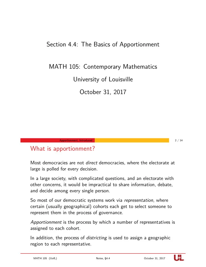
Section 4.4: The Basics of Apportionment MATH 105: Contemporary Mathematics University of Louisville October 31, 2017

Apportionment, Introduced 2 / 14

What is apportionment?

Most democracies are not direct democracies, where the electorate at large is polled for every decision. In a large society, with complicated questions, and an electorate with

• ther concerns, it would be impractical to share information, debate,

and decide among every single person. So most of our democratic systems work via representation, where certain (usually geographical) cohorts each get to select someone to represent them in the process of governance. Apportionment is the process by which a number of representatives is assigned to each cohort. In addition, the process of districting is used to assign a geographic region to each representative.

MATH 105 (UofL) Notes, §4.4 October 31, 2017

Apportionment, Introduced 3 / 14

Contexts for apportionment and districting

In some nations with parliamentary systems, voters select not a candidate by a party, and then seats in the parliament are apportioned by number of votes. In America, apportionment is done on both the national and state level by geography.

▶ Each state is apportioned a number of representatives to

Congress.

▶ Within state legislatures, representatives are often doled out

county-by-county. The subordinate process of districting is usually done by the states.Districting is a much hotter topic today than apportionment, but both can be complicated and surprisingly difficult to do fairly.

MATH 105 (UofL) Notes, §4.4 October 31, 2017 Apportionment, Introduced 4 / 14

Legal basis for apportionment

Article I, Section 2 of the US Constitution

Representatives and direct Taxes shall be apportioned among the several States which may be included within this Union, according to their respective Numbers. . . The Number of Representatives shall not exceed one for every thirty Thousand, but each State shall have at Least one Representative. This gives very little guidance; it says the number of representatives should be proportional to the population, and that there should be no more than

1 30000 times the population, but little else!

Some case law has clarified the situation somewhat; e.g. the 1964 case Wesberry v. Sanders established that each representative’s district should enclose nearly the same population. However, historically, the potential for error and unusual interpretation has been fertile ground for political scheming.

MATH 105 (UofL) Notes, §4.4 October 31, 2017

Apportionment, Introduced 5 / 14

Why should apportionment be hard?

Districting is a horrible can of worms; but why is apportionment troublesome? Sometimes it’s not; suppose we wanted to assign a 20-person proportional legislative body to the following four counties in a state with 800,000 people: County Population Smith 320,000 Burton 160,000 Clark 120,000 Ocean 200,000 20 representatives, split evenly over 800,000 people, should assign one representative to each group of 40,000 people. Logically, then, Clark County gets 3, Burton 4, Ocean 5, and Smith 8.

MATH 105 (UofL) Notes, §4.4 October 31, 2017 Apportionment, Introduced 6 / 14

Generalizing our process

In the last slide, we saw that a 20-person representative body for 800,000 people should have one representative per 40,000 people. Why? If we have n representatives, and a population P, then we want one representative per P

n people.

This number is known as the average constituency size or the standard divisor. Once we have the standard divisor, we divide each region’s population by it to get their standard quota of representatives.

MATH 105 (UofL) Notes, §4.4 October 31, 2017

Apportionment, Introduced 7 / 14

So apportionment should be really easy!

So, why not give every region its standard quota of representatives? Well, let’s suppose that the four counties measured above have unequal growth, and ten years later, have different populations: County Population Quota of reps Smith 350,000 7.37 Burton 190,000 4.00 Clark 150,000 3.16 Ocean 260,000 5.47 Our total population has grown to 950,000, for a standard divisor of 47500. So to find each county’s quota, we divide its population by 47500 above. How can we possibly select these fractional numbers of people?

MATH 105 (UofL) Notes, §4.4 October 31, 2017 Apportionment, Introduced 8 / 14

Interlude: An American history lesson

The first census was taken in 1790; at that time, the House of Representatives had 105 members. Having to “round off” non-integer quotas became a problem almost immediately in American history. Over the course of the next 150 years, America would use four different approaches to rounding off these non-integer parts. Other nations also confronted these problems, and their own solutions incuded both the same ones used in America and other approaches.

MATH 105 (UofL) Notes, §4.4 October 31, 2017

Apportionment, Introduced 9 / 14

A simple and crude approach

Recall our original plan for apportioning 20 representatives: County Population Quota of reps Smith 350,000 7.37 Burton 190,000 4.00 Clark 150,000 3.16 Ocean 260,000 5.47 If we round down, then we will assign 7 delegates to Smith County, 4 to Burton, 3 to Clark, 5 to Ocean. But this only doles out 19 reps, and we ought to have one more. The most badly cheated on their standard quota by this scheme would be Ocean County, so we’ll give them the extra delegate in recompense.

MATH 105 (UofL) Notes, §4.4 October 31, 2017 Apportionment, Introduced 10 / 14

Formalizing what we just did

So, the process we followed on the last slide can be generalized. Suppose we have a bunch of regions and a number of representatives

• N. Here’s how we might apportion them:

▶ Divide the total population by N to get the standard divisor D. ▶ Divide each region’s population by D to get their individual

standard quotas.

▶ Round down the standard quotas to get each state’s lower quota. ▶ Add up the lower quotas to determine how many representatives

are unassigned.

▶ Give out that many “bonus reps” one at a time to regions,

starting with the region whose standard quota has the largest fractional part. This approach is variously known as Hamilton’s method, Vinson’s method, the Hare-Niemeyer method, or the Method of Largest Remainders.

MATH 105 (UofL) Notes, §4.4 October 31, 2017

Apportionment, Introduced 11 / 14

Another Hamilton Method example

Let’s look at how a city council of 99 people might be apportioned among four neighborhoods: N’hood Pop.

• Std. quota

Lower quota Bonus Total Forkland 2060 10.1970 10 10 Knifeton 2080 10.2960 10 +1 11 Spoonville 7730 38.2635 38 38 Platesburg 8130 40.2435 40 40 Total 20000 99.0000 98 99 We calculate the standard divisor D = 20000

99

≈ 202.02. Then we divide each state’s population by this value D. Now we round all the quotas down. But, since we are one delegate short, we assign a bonus delegate to whichever state had the highest decimal part in its SQ.

MATH 105 (UofL) Notes, §4.4 October 31, 2017 Apportionment, Introduced 12 / 14

Tweaking that example

Suppose they decide the 99-person city council is an ungainly number, and bump it up to a nice round 100? N’hood Pop.

• Std. quota

Lower quota Bonus Total Forkland 2060 10.30 10 10 Knifeton 2080 10.40 10 10 Spoonville 7730 38.65 38 +1 39 Platesburg 8130 40.90 40 +1 41 Total 20000 100.00 98 100 The standard divisor is now 20000

100 = 200.

MATH 105 (UofL) Notes, §4.4 October 31, 2017

Apportionment, Introduced 13 / 14

A paradox, a paradox, a most ingenious paradox!

Let’s summarize how the Hamilton apportionment proposed to split

• ut either 99 or 100 representatives among those four neighborhoods:

Neighborhood 99-rep distribution 100-rep distribution Forkland 10 10 Knifeton 11 10 Spoonville 38 39 Platesburg 40 41 Total 99 100 The good people of Knifeton have cause to feel cheated by the addition of a new council member! What has happened here is a weakness of the Hamilton apportionment technique known as the Alabama Paradox.

MATH 105 (UofL) Notes, §4.4 October 31, 2017 Apportionment, Introduced 14 / 14

Pair o’ docs, pair o’ delegates

The Alabama Paradox

An apportionment technique is subject to the Alabama Paradox when an increase in the total number of representatives, without any change in population, results in one of the regions losing representatives. This paradox was discovered in 1880, when a detailed study of potential sizes for the House of Representatives determined that in a House with 299 members, Alabama would get 8, while with 300 members, it would only get 7. Nonetheless, the US continued to use the Hamilton method from 1850 to 1900. In 1900 the Paradox hit Colorado, which was apportioned three seats for every House size between 350 and 400 except for 357, at which it would only have gotten 2.

MATH 105 (UofL) Notes, §4.4 October 31, 2017