Scaling laws for products of random matrices Lois d echelle pour - - PowerPoint PPT Presentation

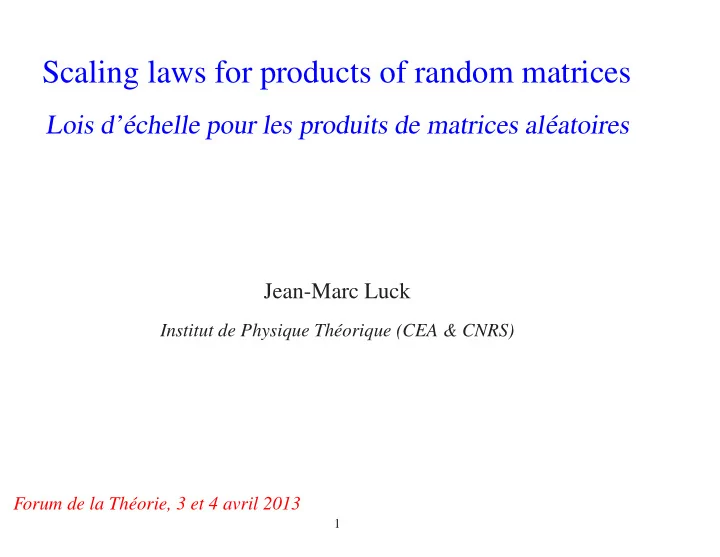
Scaling laws for products of random matrices

Lois d’´ echelle pour les produits de matrices al´ eatoires

Jean-Marc Luck

Institut de Physique Th´ eorique (CEA & CNRS) Forum de la Th´ eorie, 3 et 4 avril 2013

1

Outline

• A reminder on sums and products of random numbers
• Products of random matrices
• One-dimensional systems and products of transfer matrices
• The ferromagnetic Ising chain in a random magnetic field
• The tight-binding model in a random potential
• Band-edge scaling law
• Ubiquity of scaling laws and their classification
• Table of scaling functions

2

A reminder on sums and products of random numbers

Sum of random numbers: SN = x1 +···+xN

xi random, independent and identically distributed (i.i.d.) x = m and var x = x2 − x 2 = σ2 finite Laws of large numbers: SN is asymptotically Gaussian (normal) for large N SN = Nm and var SN = Nσ2

SN f(SN)

Nm

σN

1/2

• Sum is peaked around its mean value
• Relative fluctuations fall off as 1/

√ N

3

Product of random numbers: PN = x1 ···xN

xi i.i.d. positive random numbers

• Product peaked around typical value

P typ

N

= eN lnx lnP typ

N

= lnPN = N lnx

• Mean value of product is exponentially deep in the tail

lnx < ln x implies PN = x N = eN ln x ≫ P typ

N

PN

PN f(PN)

PN

typ

4

Products of random matrices

PN = M1 ···MN

Mi i.i.d. random matrices (say real and of size p× p ) Again peaked around typical value: P typ

N

∼ eN γ γ = lim

N→∞

1 N ln|tr PN| is Lyapunov exponent (Furstenberg, 1963)

• Describes typical value only (relevant for disordered systems)
• Generalizes explicit results lnx (numbers) and lnλ (constant matrices)
• Difficult to calculate in general (even in the 2×2 case !)

5

One-dimensional systems and products of transfer matrices

• One-dimensional system:

sequence of independent units

• Linear equations for each unit:

transfer matrix

M1 M2 M3 M4 M5 M1

Transfer-matrix formalism has proved useful in many areas

• Optics, electromagnetism, etc.
• Statistical Physics

Disordered systems: products of random transfer matrices Ferromagnetic Ising chain in a random magnetic field Tight-binding model for an electron in a random potential

6

The ferromagnetic Ising chain in a random magnetic field

H = −J∑

n

σnσn+1 −∑

n

hnσn σn = ±1 : classical Ising spins J > 0 : uniform ferromagnetic exchange constant hn : random magnetic fields (i.i.d. random variables) Canonical ensemble : partition function and free energy β = 1/T : inverse temperature ZN = ∑

{σn}

e−βH FN = −T lnZN f = lim

N→∞

FN N

7

Transfer-matrix formalism

Partition functions Z±

n

conditioned on the last spin (σn = ±) Z+

n

Z−

n

• =

eβ(J+hn) eβ(−J+hn) eβ(−J−hn) eβ(J−hn)

• M(hn)

Z+

n−1

Z−

n−1

• Chain of N spins with periodic boundary conditions

ZN = tr M(hN)···M(h2)M(h1)

8

Thermodynamic limit (N → ∞)

• Constant magnetic field

(hn = h) (Ising, 1924)

f = −T lnλ

λ is largest eigenvalue of M(h) λ = eβJ coshβh+

• sinh2 βh+e−4βJ
• Random magnetic field

( hn i.i.d.)

f = −Tγ

γ is Lyapunov exponent of matrix product M(hN)···M(h2)M(h1)

9

Statistics of free energy (ground-state energy) in disordered systems

For finite system of N sites Free energy FN = −T lnZN is a random variable (Brout, 1959)

• Quenched average

F qu

N

= −T lnZN describes properties of typical sample is physical: F qu

N

≈ N f given by Lyapunov exponent for 1D system: F qu

N

≈ −NTγ

• Annealed average

F an

N

= −T ln ZN is unphysical provides (useful) bound F an

N

> F qu

N

10

The tight-binding model in a random potential

ψn+1 +ψn−1 +Vnψn = Eψn

e

−

ψn : amplitude of wavefunction at site n E : energy eigenvalue Vn : random site energies (i.i.d. random variables)

11

Transfer-matrix formalism

ψn+1 ψn

• =

E −Vn −1 1

• M(Vn)

ψn ψn−1

• Constant potential

(Vn = V) Plane waves: ψn ∼ einq Dispersion law: tr M(V) = E −V = 2cosq

• Static random potential

( Vn i.i.d.)

• ψ typ

n

• ∼ enγ

γ is Lyapunov exponent of matrix product M(VN)···M(V2)M(V1) γ > 0 on the spectrum

12

Interpretation: localization by disorder

(Anderson, 1958)

• Eigenfunctions ψn are all localized in 1D
• Their hull falls off exponentially as |ψn| ∼ exp(±n/ξ)
• Localization length

ξ = 1 γ

50 100 150 200

n

−0.4 −0.3 −0.2 −0.1 0.1 0.2 0.3 0.4

ψn

13

Weak-disorder regime

(V = 0, V 2 ≪ 1)

• Complex characteristic exponent:

Ω = γ+iπH (Cf. Sturm, 1836) γ : Lyapunov exponent H(E) =

Z ∞

E ρ(E′)dE′ :

integrated density of states

• Perturbative result

(Thouless, 1972) E = 2coshµ (Outside the band)

Ω = µ− V 2 8sinh2 µ +···

14

Behavior of inverse localization length γ = 1/ξ

• Outside band (|E| > 2)

γ ≈ µ

• Inside band (|E| < 2, µ → iq)

γ ≈ V 2 8sin2 q

• Near band edges ( V 2 and µ small)

γ ∼ β ∼ (V 2 )1/3 E −2 ∼ β2 ∼ (V 2 )2/3

−4 −2 2 4

E

0.5 1 1.5

γ

β β

β

2

β

2

15

Band-edge scaling law

(Halperin, 1965; Derrida & Gardner, 1984) Weak disorder (V 2 ≪ 1) + Band edge (µ ≪ 1) = Scaling behavior Ω = γ+iπH = β G(x) β =

• V 2 /2

1/3, x = µ2 β2 = E −2

• V 2 /2

2/3 G(x) = e−2iπ/3 Ai′(e−2iπ/3x) Ai(e−2iπ/3x) = Ai′(x)+iBi′(x) Ai(x)+iBi(x)

• Non-trivial scaling function G(x) mixing real and imaginary parts
• Involves logarithmic derivative of special function

Here: Ai, Bi : Airy functions

16

Ubiquity of scaling laws and their classification

Quite generally: Weak disorder + ‘Interesting point’ (band edge, critical point) = Scaling behavior Our work (CLTT, 2013)

• Group SL2(R) of 2×2 real matrices with unit determinant
• Continuum limit of matrices close to unity

Outcome

• Classification of scaling functions describing Ω
• In correspondence with special functions
• Classification of types of collective behavior of 1D disordered systems

17

Universal model

(Comtet, Texier, Tourigny, 2010) Kronig-Penney model with double impurities (point-like scatterers) −d2ψ dx2 +(W(x)+U(x))ψ = ψ wn un αn xn : positions of impurities αn = xn −xn−1 : distances between impurities W(x) = ∑

n

wn

• δ2(x−xn)+δ′(x−xn)
• :

supersymmetric potential U(x) = ∑

n

un δ(x−xn) : scalar potential

18

Universal transfer matrix

M(αn,wn,un) = K(αn)A(wn)N(un)

K(α) = cosα −sinα sinα cosα

• ,

A(w) = ew e−w

• ,

N(u) = 1 u 1

• This is the Iwasawa decomposition of the group SL2(R)

(Iwasawa, 1949) Subgroup Compact Abelian Nilpotent Disorder Distance Supersymmetric Scalar

19

Continuum limit of matrices close to unity

• 3 average values

α, w, u

• 6 elements of covariance matrix

Dαα = α2 − α 2, Dαw = αw − α w, etc. simultaneously small

Main outcome

• Ω as explicit homogeneous function of these 9 parameters
• involves logarithmic derivative of special function:

Ω = ··· S ′(x) S(x)

20

Table of scaling functions

Zeros Disorder Special function S(x) 1 quadruple scalar Airy Ai(e−2iπ/3x) 2 double supersymmetric Bessel Kν(x) 2 double distance Bessel Iiλ(x) 1 double + 2 simple general potential Whittaker Wlm(x) 4 simple ‘independent’ elliptic K(k) 4 simple general hypergeometric

2F1(α,β;γ;x)

• Provides classification of types of collective behavior in 1D disordered systems
• Zeros: complex roots of instrumental fourth-degree polynomial
• Complex analysis is key novel ingredient

21

To conclude... three references

• R. Brout,

Statistical-mechanical theory of a random ferromagnetic system

• Phys. Rev. 115 (1959) 824
• JML,

Syst` emes d´ esordonn´ es unidimensionnels Collection Al´ ea Saclay (1992)

• A. Comtet, JML, C. Texier, Y. Tourigny,

The Lyapunov exponent of products of random 2×2 matrices close to the identity

• J. Stat. Phys. 150 (2013) 13

(arXiv:1208.6430)

22

Appendix: main steps of derivation

• Sequence of vectors

Xn Yn

• = Mn

Xn−1 Yn−1

• Mn = M(αn,wn,un) =

An Bn Cn Dn

• Riccati variables

Zn = Xn Yn Zn = AnZn−1 +Bn CnZn−1 +Dn Ω = lim

n→∞ ln(CnZn−1 +Dn+i0)

23

• Continuum limit:

Z(n) → continuous process dZ = V(Z) dn+

• 2D(Z) dW(n)

V(Z) = − α(Z2 +1)+2wZ + u + DααZ(Z2 +1)+2DwwZ −4DαwZ2 −2DαuZ +2Dwu 2D(Z) = Dαα(Z2 +1)2 +4DwwZ2 +Duu − 4DαwZ(Z2 +1)−2Dαu(Z2 +1)+4DwuZ

24

• Hilbert transform of invariant distribution

F(y) =

Z +∞

−∞

f(Z)dZ y−Z

• F(y) analytic in lower half plane

(Im y < 0)

• Polynomial differential equation

Q(y)F′(y)+R(y)F(y) = S(y)+2Ω These two conditions determine both F(y) and Ω

25

General case: Q(y) has 4 simple zeros

Z y2

y1

(S(y)+2Ω)

4

∏

i=1

(y−yi)ai−1 dy = 0

y1 y2 y3 y4

26

General case: the result

Ω = 1 2

• Dαα(y1 −y4)(y3 −y2)G(x)+ R(y1)

y1 −y3 −S(y1)

• G(x) = x 2F1′(1−a3,a1;a1 +a2;x)

2F1(1−a3,a1;a1 +a2;x)

x = (y1,y4;y2,y3) = (y1 −y2)(y4 −y3) (y1 −y3)(y4 −y2) =

• y2 −y1

y ∗

2 −y1

• 2

27