Run Time Complexity In typical application the total run time of a - PowerPoint PPT Presentation

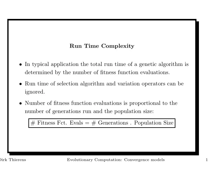
Run Time Complexity • In typical application the total run time of a genetic algorithm is determined by the number of fitness function evaluations. • Run time of selection algorithm and variation operators can be ignored. • Number of fitness function evaluations is proportional to the number of generations run and the population size: # Fitness Fct. Evals = # Generations . Population Size Dirk Thierens Evolutionary Computation: Convergence models 1

Convergence speed • Rate at which a population converges is determined by the selection pressure: – high selection pressure: fast convergence – low selection pressure: slow convergence • Size of population determines quality of solution found: – large population size: more reliable convergence – small population size: less reliable convergence • Minimal fitness function evaluations: trade-off between selection pressure and population size Dirk Thierens Evolutionary Computation: Convergence models 2

Key questions 1. How long does a GA - with a certain selection pressure - run before it converges ? 2. What is the minimal population size to ensure reliable convergence ? → ie. problem dependent, but: • we can build analytical models for simple problems, • use this as an approximation for real, complex problems, • gives insight in and guidance for designing high performant GAs. Dirk Thierens Evolutionary Computation: Convergence models 3

Models 1. First, we will build analytical models for the convergence behavior, assuming large enough ( ∞ ) populations, 2. Second, we will build analytical models for the minimal required population size, 3. Third, we will test the models on a real, complex problem (map labeling). Dirk Thierens Evolutionary Computation: Convergence models 4

Selection Intensity • To quantify the speed of convergence caused by the selection pressure we need a measure, • The field of Quantitative Genetics already works with such a measure: the selection intensity I . Dirk Thierens Evolutionary Computation: Convergence models 5

Quantitative Genetics • Quantitative genetics studies the inheritance of those differences between individuals that are quantitative rather than qualitative. • Quantitative differences have a continuous nature such as the height or the weight of the human body, whereas qualitative variation is measured in discrete units or categories such as eye color or blood type. • To characterize the evolution of the quantitative differences the following concepts are defined. • The selection progress or response to selection R ( t ) is defined as the difference between the mean fitness of the population at generation t + 1 and the mean fitness of the population at generation t . • The selection differential S ( t ) is the difference between the Dirk Thierens Evolutionary Computation: Convergence models 6

mean fitness of the parent population at generation t and the population mean fitness at generation t . The parent population is the pool of individuals remaining after selection has been applied but before the oofspring has been generated by the variation operators: S ( t ) = f ( t s ) − f ( t ) . • Assuming that the population fitness is normally distributed N ( f, σ 2 ) we can scale the selection differential by the standard deviation σ ( t ). • This scaled selection differential is called the selection intensity I ( t ). This is a dimensionless number since the standard deviation has the same units as the selection response: σ ( t ) = f ( t s ) − f ( t ) I ( t ) = S ( t ) . σ ( t ) Dirk Thierens Evolutionary Computation: Convergence models 7

• Standardizing the normal distribution ( f = 0 , σ = 1) shows that the selection intensity I is simply the expected average fitness of the population after applying the selection scheme to a population with standardized normal distributed fitness ( N (0 , 1)). • The relation between the response to selection R and the selection differential S is given by the heritability h 2 : R ( t ) = h 2 S ( t ) , or R ( t ) = h 2 σ ( t ) I ( t ) . Dirk Thierens Evolutionary Computation: Convergence models 8

Proportionate selection • Call P i ( t ) the proportion of occurrences of individual i in the population at generation t , • Individual i has fitness f i , and the mean fitness of the population at generation t is f ( t ), • Call P i ( t s ) the proportion of individual i in the parent pool after applying proportionate selection: P i ( t s ) = P i ( t ) f i . f ( t ) • The selection differential of proportionate selection is: f ( t s ) − f ( t ) S ( t ) = N � P i ( t s ) f i − f ( t ) = i =1 Dirk Thierens Evolutionary Computation: Convergence models 9

N P i ( t ) f 2 � i = − f ( t ) f ( t ) i =1 1 ( f 2 ( t ) − ( f ( t )) 2 ) = f ( t ) σ 2 ( t ) = f ( t ) (i.e. Fisher’s Fundamental Theorem of Natural Selection) • note: � N � N i =1 P i ( t ) f 2 i = f 2 ( t ) i =1 P i ( t ) f i = f ( t ); N ( X i − X ) 2 � σ 2 = N i =1 2 � N � N i =1 X 2 i =1 X i + NX i = − 2 X N N N Dirk Thierens Evolutionary Computation: Convergence models 10

2 X 2 − X = • The selection intensity I ( t ) = S ( t ) σ ( t ) of proportionate selection is thus equal to the ratio of the standard deviation of the fitness and the population mean fitness: I ( t ) = σ ( t ) f ( t ) • Observations: 1. The selection intensity of proportionate selection reduces if the fitness variance between the individuals in the population reduces and/or if the mean fitness increases. Both typically happen at later generations when the population starts to loose its diversity. The selection pressure basically disappears. Dirk Thierens Evolutionary Computation: Convergence models 11

i i 1 i 2 i 1 i 1 i 2 i 3 i 4 i 2 i 3 i 1 f i 105 101 105 105 101 93 91 101 93 105 Mean fitness f ( t ) = 100, proportions: P i ( t ), expected proportions after selection: P i ( t s ), most likely number of copies: n ( t s ). P i ( t s ) n ( t s ) i P i ( t ) i 1 0.4 0.420 4 i 2 0.3 0.303 3 i 3 0.2 0.186 2 i 4 0.1 0.091 1 ⇒ most likely no change in number of copies ! Dirk Thierens Evolutionary Computation: Convergence models 12

Selection intensity I ( t ) = σ ( t ) f ( t ) = 5 . 31 100 = 0 . 0531 Expected mean fitness after selection (i.e. the parent pool): f ( t s ) = f ( t ) + σ ( t ) I ( t ) = 100 + (5 . 31)(0 . 0531) = 100 . 28 . 2. The selection intensity of proportionate selection changes when the fitness values are transformed with a constant term, for instance when changing temperature values from Celsius to Fahrenheit (F = 1.8 C + 32). Dirk Thierens Evolutionary Computation: Convergence models 13

Truncation Selection • Selection differential S ( t ) = f ( t s ) − f ( t ), • Truncating a normal distribution at the top τ % results in a mean fitness increase that is proportional to the standard deviation: f ( t s ) − f ( t ) = C ( τ ) σ, • By the definition of the selection intensity, S ( t ) = Iσ ( t ), it follows that I ( τ ) = C ( τ ), • For a given trunction threshold τ the selection intensity is a constant equal to the mean value of the right part of a standard normal distribution ( f ( t ) = 0 , σ ( t ) = 1), truncated at the top τ %. Values can be calculated or looked up in tables: Dirk Thierens Evolutionary Computation: Convergence models 14

τ 1% 10% 20% 40% 50% 80% I ( τ ) 2.66 1.76 1.2 0.97 0.8 0.34 • Contrary to proportionate selection, the selection pressure with truncation selection remains constant and is independent of the population mean fitness and variance (this is true for all ranked-based selection methods). Dirk Thierens Evolutionary Computation: Convergence models 15

Tournament Selection • Tournament selection with tournament size s : pick s solutions at random from the population, and select the solution with the best fitness. • The selection intensity I ( s ) = ( f ( t s ) − f ( t )) /σ ( t ) is equal to the expected value of the best ranked individual of a sample from s individuals taken from the standard normal distribution ( f ( t ) = 0 and σ ( t ) = 1). • How to compute this ? → order statistics Dirk Thierens Evolutionary Computation: Convergence models 16

Order Statistics • Order statistics describes the statistical properties of a set of random variables that are ordered (or ranked) according to their value. • Assume we take a random sample of size s of a population with a certain distribution probability, and we sort the sample in increasing order of magnitude: x 1: s ≤ x 2: s ≤ . . . ≤ x s − 1: s ≤ x s : s • The i th order statistic is the random variable X i : s that represents the distribution of the corresponding value x i : s . • The probability density function p i : s ( x ) of the i th order statistic X i : s gives the probability that the i th ranked individual of a sample of size s will have a value equal to x . Dirk Thierens Evolutionary Computation: Convergence models 17

• We need to compute this for the standard normal distribution, • The probability density function is 1 e − x 2 √ φ ( x ) = 2 2 π and the cumulative distribution is � x Φ( x ) = φ ( x ) dx. −∞ • The probability density function p i : n ( x ) is given by: � s − 1 � Φ( x ) i − 1 (1 − Φ( x )) s − i φ ( x ) , p i : s ( x ) = s i − 1 • The expected value u i : s of the i th order statistic X i : s is: � + ∞ u i : s = x p i : s ( x ) dx −∞ Dirk Thierens Evolutionary Computation: Convergence models 18