Rui Carvalho, School Mathematical Sciences, QMUL QMUL: Wolfram Just - PowerPoint PPT Presentation
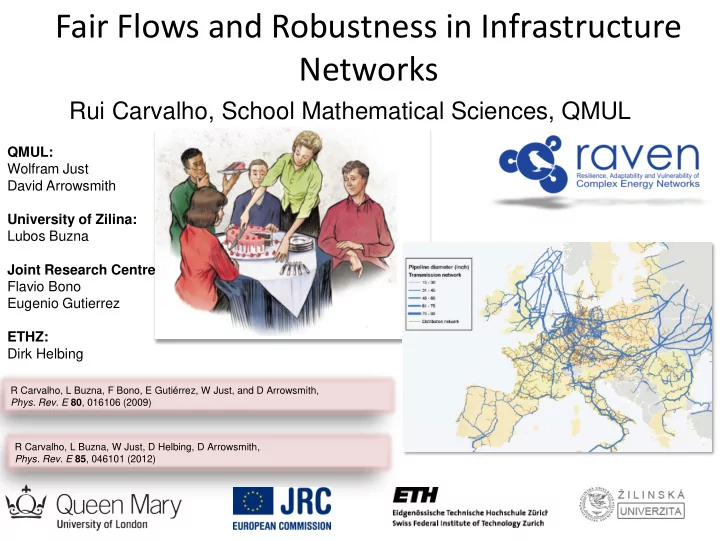
Fair Flows and Robustness in Infrastructure Networks Rui Carvalho, School Mathematical Sciences, QMUL QMUL: Wolfram Just David Arrowsmith University of Zilina: Lubos Buzna Joint Research Centre Flavio Bono Eugenio Gutierrez ETHZ: Dirk
Fair Flows and Robustness in Infrastructure Networks Rui Carvalho, School Mathematical Sciences, QMUL QMUL: Wolfram Just David Arrowsmith University of Zilina: Lubos Buzna Joint Research Centre Flavio Bono Eugenio Gutierrez ETHZ: Dirk Helbing R Carvalho, L Buzna, F Bono, E Gutiérrez, W Just, and D Arrowsmith, Phys. Rev. E 80 , 016106 (2009) R Carvalho, L Buzna, W Just, D Helbing, D Arrowsmith, Phys. Rev. E 85 , 046101 (2012)
We need to find creative uses of available infrastructure networks
Especially, when things go wrong!
Robustness
Datasets: European gas pipeline network Transmission network Complete network (d>= 15, + interconnections) 24010 nodes, 25554 links 2207 nodes, 2696 links www.platts.com
Datasets: Gas trade movements by pipeline (2007) Data collected from: www.bp.com www.iea.org
Betweenness centrality
The max-flow problem
Generalized betweenness centrality
Generalized max-flow betweenness vitality
Generalized betweenness applied to gas networks
Generalized vitality applied to gas networks
Robust infrastructure network: error tolerant to failures of high load links High Traffic Backbone + Error Tolerance = Robustness ( i.e. Good Engineering ) Rui Carvalho, Lubos Buzna, Flavio Bono, Eugenio Gutiérrez, Wolfram Just, and David Arrowsmith, Phys. Rev. E 80 , 016106 (2009)
Fair Flows The Max-Min Fairness Algorithm
From cake – cutting to fair allocation of network resources • Mathematicians have been occupied with fairness in cake-cutting since the 1940s (Steinhaus, Knaster and Banach); • But what about the similar network problem: how to allocate network capacity among users in a fair way? • Challenge: how to gain analytical insights into the fair allocation of network capacity on very large networks?
The Max-Min Fairness Algorithm
The max-min fairness problem as the lexicographic maximin problem
Max-Min Fair Flows • Consider a set of s-t pairs, each connected by a set of paths; • Each edge of a path transports the same path flow;
Max-Min Fairness [1] Typically, connections are specified by a fixed set of • paths, and one wants to allocate path flows to each of these paths. A set of path flows is max-min fair if no path flow can • be increased without simultaneously decreasing another path flow that is already less or equal to the former. to increase a path flow you need to decrease that is already smaller another path flow • D. Bertsekas and R. Gallager, Data Networks, Prentice-Hall, 1987 • J. Kleinberg, Y. Rabani and E. Tardos, Journal of Computer and Systems Sciences 63 , 2 (2001)
Max-min Fairness Algorithm: First Step [2]
Max-min Fairness Algorithm: First Step The crucial elements of the algorithm
Max-min Fairness Algorithm: Second Step
Max-min Fairness Algorithm: Second Step (cont.)
Max-Min Fairness in Nearest Neighbour Networks
Assumptions [3] Consider a set of s-t pairs, each connected by a set of • paths; Each edge of a path transports the same path flow ; • Furthermore, we consider transport: – over shortest paths (path counting) – on networks with uniform edge capacity (path counting) – on regular grids (analytical results) – on 1 s-t pair (analytical results);
Max-Min Fairness: Assumptions [3] Consider a set of s-t pairs, each connected by a set of • paths; Each edge of a path transports the same path flow ; • Furthermore, we consider transport: – over shortest paths (path counting) – on networks with uniform edge capacity (path counting) – on regular grids (analytical results) – on 1 s-t pair (analytical results);
[4] K-nearest neighbour networks Two ways of measuring distance: difference d between the • indexes of s and t Shortest path distance L • between s and t
Number of shortest paths from s to t [5] A shortest path is an • arrangement of the K/2 rows into L-1 ‘stars’ and K/2-1 ‘bars’; Each * marks a row and each | • marks a change of consecutive rows in the path, e.g. *|*||*; So the number of shortest • paths between s and t is given by the number of ways to distribute L-1 identical balls ( * ) the into K/2 distinct bags (rows), where each row can get any number of balls:
Number of s-t shortest paths as a function of s-t distance on K-nearest neighbour graphs Determining the sink inflow on a K -nearest neighbour network as the s-t distance d is varied is reduced to the problem of calculating sink inflows for 𝑒 𝑛𝑗𝑜 (K,L) .
Path Counting Methods
Path Counting Methods
Relation between path counting and path [7] flows number of unsaturated paths found recursively
[8] The path flow increment at the last iteration ∆𝑔 (𝑗) 𝑠 (𝑗) = 𝑗 ∆𝑔 (𝑗) 𝑘=1 𝑠 (𝑗) → 1 tells us that that path flows are dominated by ∆𝑔 at the last iteration
From path counting to path flows and back • Path counting methods are still valid when : – we have bottlenecks at s and t for all rows above the current; – We have a ‘chain’ of bottlenecks on one row (and at the symmetric row), followed by bottlenecks at s and t . • Our methods stop working when there is a gap in the row of two consecutive bottlenecks; • So what can we conclude from this?
Sink Inflow [11] Fairness implies at least 50% loss of sink inflow compared to max-flow
Diversity of the number of paths [6] crossing edges as d is varied The pattern of intersections among these paths constraints the solution of the MMF flow, because the paths share the capacity of the edges they cross L=5
Parameter Space Diagram [12] analytical results semi-analytical procedure well understood up to ‘gap’ layer w ell understood up to ‘gap’ layer
How do we generalise the path counting from the solid border to the dashed border? Instead of knowing the position of bottlenecks, we • search for them; Once we find their location, we use path counting • results as before; This works as long as there are no gaps in the row of • bottlenecks. TWO CASES: i) all bottlenecks are edges of s or t until iteration i-1 , • but bottleneck at iteration i is not an edge of s or t ; We show theoretically that • is minimum on a horizontal edge. This simplifies the search. ii) Case i) was valid up to iteration j<i . • Search over horizontal edges still valid, as long as there are no – gaps in the rows of consecutive bottlenecks. We get a chain of horizontal bottlenecks followed by a – bottleneck at s or t .
Can power-law flows be fair? [13] Region defined by the • solid line in the parameter diagram: histogram of path flows well described by power law with slope -1; Region defined by the • dashed line: slight deviation from power law caused by ‘chains’ of bottlenecks.
Why do we get power-laws? Two factors • a) the path flows are dominated by the path flow increments at the last iteration (when the paths are saturated): b) when L is large, the number of s-t • shortest paths that are saturated at iteration i is of the order of magnitude of the number of s-t shortest paths in the residual network:
Conclusions • Max-min fairness requires a big sacrifice in network throughput (at least 50% in nearest- neighbour networks); • Unexpected result: power law allocations can be fair ! • The location of bottlenecks is trivial for L small, but the pattern seem more and more elaborate as L increases for K large – how elaborate can it get as L is increased? • We are currently finishing a paper on proportionally fair allocations on the European gas pipeline network , and I will be showing the results within the next few months. Rui Carvalho, Lubos Buzna, Wolfram Just, Dirk Helbing, David Arrowsmith, Phys. Rev. E 85 , 046101 (2012)
Recommend
More recommend
Explore More Topics
Stay informed with curated content and fresh updates.

