Routing without Flow Control Costas Busch Rensselaer Polytechnic - PowerPoint PPT Presentation
Routing without Flow Control Costas Busch Rensselaer Polytechnic Institute Maurice Herlihy Brown University Roger Wattenhofer Microsoft Research 1 The network: n mesh n n n Discrete time Bi-directional links At most one
Routing without Flow Control Costas Busch Rensselaer Polytechnic Institute Maurice Herlihy Brown University Roger Wattenhofer Microsoft Research 1
The network: n mesh n n n • Discrete time • Bi-directional links • At most one packet per link direction 2
Dynamic Routing: Packets are injected continuously destination 3
A new packet can be injected when there is a free link : A link direction is empty 4
Most dynamic routing algorithms use flow control : Don’t utilize all the free links Disadvantage: Network is under-utilized 5
Our Routing Algorithm: • No flow control • Utilizes all the free links Advantage: Network is fully-utilized 6
Features of our algorithm: • Dynamic • Hot potato • Optimal delivery time: ( n ) O • Injection time guaranty: ( n ) O 7
Talk Outline The Algorithm Time Analysis Stability Future Work 8
Hot-Potato Routing: • Nodes are buffer-less • Packets are immediately forwarded 9
Conflicts 10
Conflicts Conflict 11
Conflicts Deflected 12
Packet states: Priorities: Running high Excited Active Sleeping low 13
Sleeping packet destination Random destination 14
Sleeping packet destination Follows a path to destination 15
Sleeping packet becomes Active with n probability 1 n n 16
Active packet Follows a greedy path 17
Active packet Follows a greedy path 18
Active packet A conflict situation 19
Active packet Conflict A conflict situation 20
Active packet Deflected A conflict situation 21
Active packet becomes Deflected Excited with probability 1 p n A conflict situation 22
Excited packet Follows a one-bend path 23
Excited packet becomes Running Follows a one-bend path 24
Running packet Follows a one-bend path 25
Talk Outline The Algorithm Time Analysis Stability Future Work 26
Good condition for a column: at most non-sleeping packets 10 n with destination in the column 27
Expected delivery time for one packet: n (when the destination column is in good condition) 28
Initially a packet is sleeping In expected time steps n becomes active We will show: An active packet is delivered in expected time steps O n 29
Interrupting a one-bend path Excited Time 1 30
Interrupting a one-bend path Running Time 2 31
Interrupting a one-bend path Excited Running Time 2 32
Interrupting a one-bend path Running Running Time 3 33
Interrupting a one-bend path Running conflict Running Time 4 34
Interrupting a one-bend path deflected Active Running Time 5 35
No interruption probability: ( m 1 p ) Excitement probability Number of non-sleeping packets with destinations in same column 36
No interruption probability: p m ) ( 1 c 1 n constant n (when the destination column is in good condition) 37
Probability of success after a deflection: 1 p c n Expected number of deflections until success: n Expected delivery time for an active packet: O n 38
Talk Outline The Algorithm Time Analysis Stability Future Work 39
Divide time in time periods: t 6 n Examine the condition of a column 40
1 time period e n 1 e n Good condition Bad condition 10 m n 10 m n 41
1 time period e n 1 e n Good condition Bad condition ne 10 m n n 10 m n 1 ne n 4n time periods 42
1 time period e n 1 e n Good condition Bad condition 10 m n 10 m n 43
Proof Outline In a time period: • At most new non-sleeping 2 n packets are generated with destinations in the column • At least non-sleeping packets 2 n are delivered (if ) 8 m n 44
Good condition Bad condition ne 10 m n n 10 m n 1 ne n 4n time periods 45
Proof Outline In a time period: • At most new non-sleeping 2 n packets are generated with destinations in the column • At least non-sleeping packets 3 n are delivered 46
Consequences: • Most of the time, the columns are in good condition • Each packet is delivered in expected time n 47
Talk Outline The Algorithm Time Analysis Stability Future Work 48
• Arbitrary network topologies • De-randomization: Determistic destinations No randomized algorithm • Small number of packets 49
Recommend
More recommend
Explore More Topics
Stay informed with curated content and fresh updates.
