Risk and Ambiguity in Models of Business Cycles Dave Backus, Axelle - - PowerPoint PPT Presentation

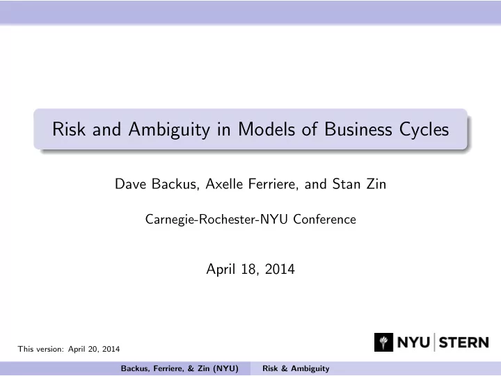
Risk and Ambiguity in Models of Business Cycles

Dave Backus, Axelle Ferriere, and Stan Zin

Carnegie-Rochester-NYU Conference

April 18, 2014

This version: April 20, 2014 Backus, Ferriere, & Zin (NYU) Risk & Ambiguity

The “Great Recession” and its aftermath

Backus, Ferriere, & Zin (NYU) Risk & Ambiguity

The “Great Recession” and its aftermath

Backus, Ferriere, & Zin (NYU) Risk & Ambiguity

The “Great Recession” and its aftermath

Backus, Ferriere, & Zin (NYU) Risk & Ambiguity

What happened?

What we see

◮ Much deeper recession than usual ◮ Longer recovery — maybe slower, too

Like Kydland-Prescott with productivity shocks?

◮ Relative magnitudes look right ◮ Comovements look right ◮ But... measured productivity didn’t fall very much More

What’s missing?

Backus, Ferriere, & Zin (NYU) Risk & Ambiguity

What happened?

Backus, Ferriere, & Zin (NYU) Risk & Ambiguity

What happened?

Marco Buti, Director General of the European Commission

Economic theory suggests that uncertainty has a detrimental effect on economic activity by giving agents the incentive to postpone investment, consumption and employment decisions until uncertainty is resolved, and by pushing up the cost of capital through increased risk premia.

Backus, Ferriere, & Zin (NYU) Risk & Ambiguity

What happened?

Nick Bloom

The onset of the Great Recession was accompanied by a massive surge in uncertainty. The size of this uncertainty shock was so large it potentially accounted for around one third of the 9% drop in GDP versus trend during 2008-2009.

Backus, Ferriere, & Zin (NYU) Risk & Ambiguity

What we do

Take a streamlined business cycle model Ask: How does uncertainty affect the dynamics of output, consumption, and investment?

◮ How are business cycle properties affected by fluctuations in

uncertainty?

◮ Can “uncertainty shocks” magnify downturns or produce slow

recoveries?

Potential issues: Barro-King, Tallarini

Backus, Ferriere, & Zin (NYU) Risk & Ambiguity

Modeling ingredients

Streamlined business cycle model

• Recursive preferences
• Unit root in productivity
• Fixed labor supply

With fluctuations in uncertainty

• Risk (stochastic volatility)
• Ambiguity (unobservable long-term growth)

Backus, Ferriere, & Zin (NYU) Risk & Ambiguity

Preview of results

Solution method

Transparent loglinear approximation Checked numerically

Business cycle properties

Separation property Intertemporal elasticity of substitution vs. risk aversion Risk vs. ambiguity

Backus, Ferriere, & Zin (NYU) Risk & Ambiguity

Risk and uncertainty

Recursive references Ut = V [ct, µt(Ut+1)] = [(1 − β)cρ

t + βµt(Ut+1)ρ]1/ρ

µt(Ut+1) = [Et(Uα

t+1)]1/α

V , µt homogeneous of degree one, α, ρ < 1, σ = 1/(1 − ρ) Stochastic structure of productivity at log gt = log(at/at−1) = log g + e⊤xt (“productivity growth”) xt+1 = Axt + v 1/2

t

Bw1t+1 (“news”) vt+1 = (1 − ϕv)v + ϕvvt + τw2t+1 (“risk”) (w1t, w2t) = iid standard normals

Backus, Ferriere, & Zin (NYU) Risk & Ambiguity

Stationarity

Bellman equation J(kt, xt, vt, at) = max

ct

V

• ct, µt[J(kt+1, xt+1, vt+1, at+1)]
• s.t.

kt+1 = f (kt, atn) − ct plus shocks & initial conditions Assume f hd1: f (k, an) = kω(an)1−ω + (1 − δ)k Rescaled Bellman equation [˜ kt = kt/at, ˜ ct = ct/at] J(˜ kt, xt, vt, 1) = max

˜ ct

V

• ˜

ct, µt[gt+1J(˜ kt+1, xt+1, vt+1, 1)]

• s.t.

gt+1˜ kt+1 = f (˜ kt, n) − ˜ ct plus shocks & initial conditions

More Backus, Ferriere, & Zin (NYU) Risk & Ambiguity

Recursive business cycle model

Bellman equation Jt = max

˜ ct

[(1 − β)˜ cρ

t + βµt(gt+1Jt+1)ρ]1/ρ

s.t. ˜ kt+1 = [f (˜ kt, n) − ˜ ct]/gt+1 plus shocks & initial conditions First-order and envelope conditions (1 − β)˜ cρ−1

t

= βµt(gt+1Jt+1)ρ−αEt[(gt+1Jt+1)α−1Jkt+1] Jkt = J1−ρ

t

βµt(gt+1Jt+1)ρ−αEt[(gt+1Jt+1)α−1Jkt+1]fkt ⇒ (1 − β)˜ cρ−1

t

= Jρ−1

t

Jkt/fkt

Backus, Ferriere, & Zin (NYU) Risk & Ambiguity

Loglinearization strategy

Goal: loglinear decision rule and (controlled) law of motion log ˜ ct = hck log ˜ kt + h⊤

cxxt + hcvvt

log ˜ kt+1 = hkk log ˜ kt + h⊤

kxxt + hkvvt − log gt+1

Dynamic programming version of Campbell (JME, 1994) Loglinearization around the stochastic steady-state

Backus, Ferriere, & Zin (NYU) Risk & Ambiguity

Loglinear approximation

Guess loglinear value function log Jt = pk log ˜ kt + p⊤

x xt + pvvt + p0

Loglinearize capital’s marginal product and law of motion log fkt = λr log ˜ kt + λ0 log ˜ kt+1 = λk log ˜ kt − λc log ˜ ct + λ1 − log gt+1

More Backus, Ferriere, & Zin (NYU) Risk & Ambiguity

Loglinearized policies 1

The law of motion for capital is log ˜ kt+1 = hk0 + hkk log ˜ kt + h⊤

kxxt + hkvvt − log gt+1

hkk = λk − λc[σ + (1 − σ)pk + σλr] h⊤

kx = −λc(1 − σ)p⊤ x

hkv = −λc(1 − σ)pv Tallarini (σ = 1)

Backus, Ferriere, & Zin (NYU) Risk & Ambiguity

Loglinearized policies 2

The law of motion for capital is log ˜ kt+1 = hk0 + hkk log ˜ kt + h⊤

kxxt + hkvvt − log gt+1

hkk = λk − λc[σ + (1 − σ)pk + σλr] h⊤

kx = −λc(1 − σ)p⊤ x

hkv = −λc(1 − σ)pv Separation property

◮ hkk is independent of risk and risk aversion.

ρpk − 1 − λr =

• ρpk − 1
• λk − λc[(1 − σ)pk + σ(1 + λr)]
• .

Backus, Ferriere, & Zin (NYU) Risk & Ambiguity

Loglinearized policies 3

The law of motion for capital is log ˜ kt+1 = hk0 + hkk log ˜ kt + h⊤

kxxt + hkvvt − log gt+1

hkk = λk − λc[σ + (1 − σ)pk + σλr] h⊤

kx = −λc(1 − σ)p⊤ x

hkv = −λc(1 − σ)pv Exposure to shocks (xt, vt)

◮ If σ < 1, an increase in vt lowers consumption ◮ Magnitude depends on α (pv ∝ α) Backus, Ferriere, & Zin (NYU) Risk & Ambiguity

Loglinear approximation

3 3.1 3.2 3.3 3.4 3.5 3.6 3.7 3.8 3 3.1 3.2 3.3 3.4 3.5 3.6 3.7 3.8 log k(t) log k(t+1) numerical solution 0.03 0.06 0.09 0.12 0.15 density measure

Backus, Ferriere, & Zin (NYU) Risk & Ambiguity

Loglinear approximation

3 3.1 3.2 3.3 3.4 3.5 3.6 3.7 3.8 3 3.1 3.2 3.3 3.4 3.5 3.6 3.7 3.8 log k(t) log k(t+1) numerical solution loglinear approximation 0.03 0.06 0.09 0.12 0.15 density measure

Backus, Ferriere, & Zin (NYU) Risk & Ambiguity

Recursive business cycle model: benchmark parameters

Parameter Value Comment Preferences ρ −1 arbitrary α −9 arbitrary β — chosen to hit k/y = 10 (quarterly) Technology ω 1/3 Kydland and Prescott (1982, Table I), rounded off δ 0.025 Kydland and Prescott (1982, Table I) Productivity growth log g 0.004 Tallarini (2000, Table 4) e 1 normalization A no predictable component (“news”) B 1 normalization v 1/2 0.015 Tallarini (2000, Table 4), rounded off ϕv 0.95 arbitrary τ 0.74 × 10−5 makes v three standard deviations from zero

Backus, Ferriere, & Zin (NYU) Risk & Ambiguity

Recursive business cycle model: properties

US Data Additive Recursive Recursive Parameter changes ρ = −1 ρ = −1 ρ = 1/3 α = −1 α = −9 α = −9 Standard deviations (%) Output growth 1.04 1.00 1.00 1.01 Consumption growth 0.55 0.69 0.71 1.34 Investment growth 2.79 1.91 1.61 4.54 Correlations with output growth Consumption growth 0.52 0.99 0.96 –0.23 Investment growth 0.65 0.99 0.94 0.35 Asset returns Maximum risk premium > 0.01 ??

Backus, Ferriere, & Zin (NYU) Risk & Ambiguity

What did we learn?

Separation property

• Responses to endogenous state variables are independent of risk

aversion

IES vs. risk-aversion

• IES changes signs and correlations
• Risk aversion changes magnitudes

Backus, Ferriere, & Zin (NYU) Risk & Ambiguity

Risk and ambiguity

Divide the state in two: st = (s1t, s2t) Ambiguity (Klibanoff, Marinacci, & Mukerji; Ju & Miao) risk = p1t(s1t+1|s2t+1, It) ambiguity = p2t(s2t+1|It) Two-part certainty equivalent µ1t(Ut+1) =

• E1t(Uα

t+1)

1/α µ2t[µ1t(Ut+1)] =

• E2t[µ1t(Ut+1)]γ)

1/γ α controls risk aversion, γ < α controls ambiguity aversion

Backus, Ferriere, & Zin (NYU) Risk & Ambiguity

Loglinear structure of consumption equivalents

Log of CE with risk

log c ∼ N(κ1, κ2) log E(cα) = ακ1 + α2κ2/2 log µ(c) = κ1 + ακ2/2

Log of CE with ambiguity about mean

log c ∼ N(ν, κ2) (risk) ν ∼ N(κ1, κ3) (ambiguity) log µ(c) = κ1 + ακ2/2 + γκ3/3

Backus, Ferriere, & Zin (NYU) Risk & Ambiguity

Learning about the mean

Consider two stochastic processes

• xt the mean growth rate (unobservable, persistent)
• gt the realized growth rate (observable)

xt+1 = ϕxt + σ2w2,t+1 log gt = log g + xt + σ1w1,t

Learning: Kalman filter

ˆ xt+1 = ϕ σ2

1

At + σ2

1

ˆ xt + ϕ At At + σ2

1

log(gt/g) At+1 = σ2

2 +

φ2At At + σ2

1

σ2

1

Steady-state constant volatility ˆ xt+1 ∼ N(ˆ xt, A)

Backus, Ferriere, & Zin (NYU) Risk & Ambiguity

Stochastic learning

Add stochastic volatility vt to the signal

xt+1 = ϕxt + σ2w2,t+1 vt+1 = (1 − ϕv)¯ v + ϕvvt + σ3w3,t+1 log gt+1 = log g + xt+1 + v 1/2

t

w1,t+1

Learning: Kalman filter

ˆ xt+1 = ϕ vt−1 At + vt−1 ˆ xt + ϕ At At + vt−1 log (gt/g) At+1 = σ2

2 +

ϕ2At At + vt−1 vt−1 Fluctuating uncertainty

Backus, Ferriere, & Zin (NYU) Risk & Ambiguity

What did we learn?

What does risk + ambiguity add to a RBC model?

◮ Affects responses of variables to shocks ◮ But not internal dynamics of capital (separation property)

Feedback from endogenous variables to uncertainty?

Backus, Ferriere, & Zin (NYU) Risk & Ambiguity

Related work (some of it)

Recursive preferences

◮ Kreps & Porteus; Epstein & Zin; Weill

Recursive business cycles

◮ Tallarini; Campanale, Castro, & Clementi; Rubio & Villaverde;

Liu & Miao

Ambiguity and business cycles

◮ Klibanoff, Marinacci, & Mukerji; Jahan-Parvar & Miao; Ju &

Miao; Ilut & Schneider

Approximation methods

◮ Hansen & Sargent; Anderson, Hansen, McGrattan, & Sargent;

Campbell; Kaltenbrunner and Lochstoer; Malkhozov

Backus, Ferriere, & Zin (NYU) Risk & Ambiguity

Scaling

Back

Rescaled Bellman equation J(˜ kt, xt, θt) = max

˜ ct

V

• ˜

ct, µt[gt+1J(˜ kt+1, xt+1, θt+1)]

• s.t.

gt+1˜ kt+1 = f (˜ kt, n) − ˜ ct plus shocks & initial conditions Let K ≡ gt+1˜ kt+1. Then,

J(˜ kt, xt, θt) = max

K

V

• f (˜

kt, n) − K

• , µt
• gt+1J

K gt+1 , xt+1, θt+1, 1

• plus shocks & initial conditions

Backus, Ferriere, & Zin (NYU) Risk & Ambiguity

Productivity

Backus, Ferriere, & Zin (NYU) Risk & Ambiguity

Loglinear approximation

Back

Guess loglinear derivative of value function, then integrate log Jkt = log p1 + (pk − 1) log ˜ kt + p⊤

x xt + pvvt

Jkt = p1˜ kpk−1

t

exp(p⊤

x xt + pvvt)

⇒ Jt = p0 + (p1/pk)˜ kpk

t exp(p⊤ x xt + pvvt)

Backus, Ferriere, & Zin (NYU) Risk & Ambiguity

Loglinear approximation

Back

Guess loglinear derivative of value function, then integrate log Jkt = log p1 + (pk − 1) log ˜ kt + p⊤

x xt + pvvt

Jkt = p1˜ kpk−1

t

exp(p⊤

x xt + pvvt)

⇒ Jt = p0 + (p1/pk)˜ kpk

t exp(p⊤ x xt + pvvt)

Not loglinear: loglinearize the value function log Jt = constant + d(log p1 + pk log ˜ kt + p⊤

x xt + pvvt)

with d = (J − p0)/J [= 1 if p0 = 0]

Backus, Ferriere, & Zin (NYU) Risk & Ambiguity

Loglinear approximation

Back

Guess loglinear derivative of value function, then integrate log Jkt = log p1 + (pk − 1) log ˜ kt + p⊤

x xt + pvvt

Jkt = p1˜ kpk−1

t

exp(p⊤

x xt + pvvt)

⇒ Jt = p0 + (p1/pk)˜ kpk

t exp(p⊤ x xt + pvvt)

Not loglinear: loglinearize the value function log Jt = constant + d(log p1 + pk log ˜ kt + p⊤

x xt + pvvt)

with d = (J − p0)/J [= 1 if p0 = 0] Numerically, d is really close to 1...

Backus, Ferriere, & Zin (NYU) Risk & Ambiguity

Loglinearized policies

Back

The law of motion for capital has the form log ˜ kt+1 = hk0 + hkk log ˜ kt + h⊤

kxxt + hkvvt − log gt+1

with hkk = λk − λchck = λk − λc[σ + (d − σ)pk + σλr] h⊤

kx

= −λch⊤

cx

= −λc(d − σ)p⊤

x

hkv = −λchcv = −λc(d − σ)pv.

Backus, Ferriere, & Zin (NYU) Risk & Ambiguity

Separation property

Back

The envelope condition gives us the following quadratic expression for pk

• ρpk − 1 − λr
• =
• ρpk − 1
• λk − λc[(1 − σ)pk + σ(1 + λr)]
• .

Strategy: adjust β, not the steady-state

◮ Fix all parameters but β and α; ◮ Pick an α, then adjust β s.t. k is equal to some number. Backus, Ferriere, & Zin (NYU) Risk & Ambiguity