Risk Aggregation, Motivation Numerical Stability and a CreditRisk - PowerPoint PPT Presentation
Outline of Presentation Risk Aggregation, Motivation Numerical Stability and a CreditRisk + and extensions Variation of Panjers Recursion Panjers recursion Numerical stability Winter School on Mathematical Finance and
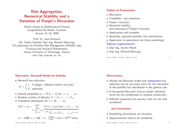
Outline of Presentation Risk Aggregation, • Motivation Numerical Stability and a • CreditRisk + and extensions Variation of Panjer’s Recursion • Panjer’s recursion • Numerical stability Winter School on Mathematical Finance and extensions of Panjer’s recursion CongresHotel De Werelt, Lunteren • Applications and examples January 21–23, 2008 • Quantiles, expected shortfall, risk contributions Prof. Dr. Uwe Schmock • Application to operational risk (time permitting) (Dr. Stefan Gerhold, Dipl.-Ing. Richard Warnung) Software implementation: CD-Laboratory for Portfolio Risk Management (PRisMa Lab) • Dipl.-Ing. Severin Resch Financial and Actuarial Mathematics • Dipl.-Ing. Richard Warnung Vienna University of Technology, Austria www.fam.tuwien.ac.at c � Jan. 23, 2008, U. Schmock, FAM, TU Vienna 2 Motivation: Bernoulli Model for Defaults Observations . . . • Bernoulli loss indicators • Already the Bernoulli model with independent loss � 1 indicators has far too many terms for the calculation if obligor i defaults (within one year), N i = of the portfolio loss distribution in the general case. 0 otherwise. • In the general Bernoulli mixture model, individual • Default probability p i = P ( N i = 1) for i = 1 , . . . , m . terms are too complicated to compute numerically. • Random number of defaults N = N 1 + · · · + N m . • Different exposures and recovery rates are not even • Probability distribution for n ∈ { 0 , . . . , m } considered. � � � P ( N = n ) = N i = 1 I ( i ) for i = 1 , . . . , m P . . . and Conclusions � �� � I ⊂{ 1 ,...,m } if ind. ( � i ∈ I p i ) � | I | = n = i ∈{ 1 ,...,m }\ I (1 − p i ) • Simplifying assumptions are necessary. � 1000 � ≈ 6 . 4 × 10 139 terms m = 1000, n = 100 = ⇒ • Approximations need to be considered. 100 c c � Jan. 23, 2008, U. Schmock, FAM, TU Vienna 3 � Jan. 23, 2008, U. Schmock, FAM, TU Vienna 4
Poisson Approximation Simple Poisson Model for Defaults • X 1 , . . . , X m independent default 0-1-indicators • Number N i of defaults of obligor i ∈ { 1 , . . . , m } • Intensity λ = � m i =1 p i with p i = P ( X i = 1) • Assume N i ∼ Poisson( λ i ) for all i ∈ { 1 , . . . , m } • Number of default events W = � m i =1 X i (several defaults of an obligor possible). • Total variation distance • Assume independence of N 1 , . . . , N m . d TV ( µ, ν ) = sup | µ ( A ) − ν ( A ) | • Random number of defaults N = N 1 + · · · + N m . A ⊂ N 0 Quality of Poisson approximation (Barbour/Hall, 1984): • N ∼ Poisson( λ ) with λ = λ 1 + · · · + λ m , i.e., m ≤ 1 − e − λ � P ( N = n ) = λ n � � p 2 d TV L ( W ) , Poisson( λ ) n ! e − λ for all n ∈ N 0 . i λ i =1 For full proof with Stein–Chen method, see e.g. Barbour, Holst ⇒ P ( N > 20) ≤ 2 × 10 − 9 . • m = 20, λ i = 0 . 2 = and Janson: Poisson Approximation, Clarendon Press (1992). c c � Jan. 23, 2008, U. Schmock, FAM, TU Vienna 5 � Jan. 23, 2008, U. Schmock, FAM, TU Vienna 6 Introduction to CreditRisk + , Standard Features Extensions of CreditRisk + • Stochastic losses of individual obligors are allowed, • Developed by Credit Suisse First Boston. distribution may depend on the causing risk factor. • Actuarial model for the aggregation of credit risks. • Risk groups with dependent stochastic losses given default are possible. • Based on the Poisson approximation of individual de- faults and the divisibility of the Poisson distribution. • Risk factors for default frequencies may be dependent. • Risk contributions of obligors can be calculated. • Allows for deterministic exposures/recovery rates. • Even with all the extensions, the probability • Several independent risk factors for dependence of generating function ϕ L of the credit portfolio loss L default frequencies can be considered. is available in closed form. → No Monte Carlo simulation, no stochastic error! • Probability generating function ϕ L of the credit portfolio loss L is available in closed form. • Distribution of L and risk contributions can be calcu- → No Monte Carlo simulation, no stochastic error! lated from ϕ γ,L with a numerically stable algorithm. c c � Jan. 23, 2008, U. Schmock, FAM, TU Vienna 7 � Jan. 23, 2008, U. Schmock, FAM, TU Vienna 8
Input Parameters of CreditRisk + (Extended Version) Input Parameters of CreditRisk + (Cont.) • Number of obligors m ∈ N . For every group g ∈ G we need • the (one year) default probability p g ∈ [0 , 1], • Basic loss unit E > 0. • the susceptibility w g, 0 ∈ [0 , 1] to idiosyncratic risk, • Number K ∈ N 0 of risk factors or non-idiosyncratic, • the susceptibilities w g,k ∈ [0 , 1] to risk factors k ∈ (independent) default causes. { 1 , . . . , K } , • Relative default variances σ 2 k > 0 of risk factors • the multivariate probability distributions k ∈ { 1 , . . . , K } . 0 on N g Q g,k = { q g,k,µ } µ ∈ N g 0 describing the stochastic losses of all the obligors i ∈ g in multiples of the • Collection G of nonempty subsets of all obligors basic loss unit E in case the risk group g defaults { 1 , . . . , m } , called risk groups. due to risk k ∈ { 0 , . . . , K } . c c � Jan. 23, 2008, U. Schmock, FAM, TU Vienna 9 � Jan. 23, 2008, U. Schmock, FAM, TU Vienna 10 Further Assumptions, Notation Notation for Default Events of Risk Groups Number of defaults for every risk group g ∈ G : • We assume that every obligor i ∈ { 1 , . . . , m } belongs • N g, 0 due to idiosyncratic risk, to at least one group g ∈ G . • Let G i := { g ∈ G | i ∈ g } denote the set of all risk • N g,k due to risk k ∈ { 1 , . . . , K } , groups to which obligor i ∈ { 1 , . . . , m } belongs, by • N g := � K k =0 N g,k total. assumption G i � = ∅ . • We assume that for each group the susceptibilities Notation for Default Events of Individual Obligors (also called weights) exhaustively describe the risk Number of defaults for every obligor i ∈ { 1 , . . . , m } factors. That is, for all g ∈ G , • N i, 0 := � g ∈ G i N g, 0 due to idiosyncratic risk, K � • N i,k := � w g,k = 1 . g ∈ G i N g,k due to risk k ∈ { 1 , . . . , K } , k =0 • N i := � K k =0 N i,k = � g ∈ G i N g total. c c � Jan. 23, 2008, U. Schmock, FAM, TU Vienna 11 � Jan. 23, 2008, U. Schmock, FAM, TU Vienna 12
Notation for Stochastic Losses Loss Attributed to Obligor i ∈ { 1 , . . . , m } • Due to group g ∈ G i and risk k ∈ { 0 , . . . , K } Loss at default number n ∈ N of risk group g ∈ G due to risk factor k ∈ { 1 , . . . , K } or idiosyncratic risk k = 0 N g,k � L g,i,k := L g,i,k,n . • L g,i,k,n part attributed to obligor i ∈ g n =1 • L g,k,n := � • Due to risk k ∈ { 0 , . . . , K } i ∈ g L g,i,k,n loss of entire group � L i,k := L g,i,k . Summation over default numbers, risks and groups: g ∈ G i • L g,k := � N g,k n =1 L g,k,n total loss of the group for risk k • Total attributed loss K • L g := � K k =0 L g,k total loss of the risk group � L i := L i,k . • L = � k =0 g ∈ G L g portfolio loss c c � Jan. 23, 2008, U. Schmock, FAM, TU Vienna 13 � Jan. 23, 2008, U. Schmock, FAM, TU Vienna 14 Probabilistic Assumptions Probabilistic Assumptions (Cont.) for the Extended Version of CreditRisk + • The group default numbers { N g, 0 } g ∈ G due to id- iosyncratic risk are independent from one another • For every group g ∈ G and every risk k ∈ { 0 , . . . , K } , the sequence of N g and from all other random variables. 0 -valued random vectors ( L g,i,k,n ) i ∈ g • The risks factors Λ 1 , . . . , Λ K are independent, with n ∈ N is i.i.d. and independent of all other ran- each one gamma distributed with E [Λ k ] = 1 and dom variables, with distribution Var(Λ k ) = σ 2 k > 0, i.e., α k = β k = 1 /σ 2 k . µ ∈ N g P ( L g,i,k, 1 = µ i for all i ∈ g ) = q g,k,µ , 0 . • For all groups g ∈ G and risks k ∈ { 1 , . . . , K } , a.s. L ( N g,k | Λ 1 , . . . , Λ K ) = L ( N g,k | Λ k ) • For each group g ∈ G , the number N g, 0 of idiosyn- catic defaults is Poisson distributed according to the a.s. = Poisson( λ g w g,k Λ k ) . Poisson intensity λ g and the susceptibility w g, 0 , i.e., • Conditionally on Λ 1 , . . . , Λ K , the risk factor based de- � � � N g, 0 ∼ Poisson( λ g w g, 0 ) for every g ∈ G. faults N g,k � g ∈ G, k ∈ { 1 , . . . , K } are independent. c c � Jan. 23, 2008, U. Schmock, FAM, TU Vienna 15 � Jan. 23, 2008, U. Schmock, FAM, TU Vienna 16
Recommend
More recommend
Explore More Topics
Stay informed with curated content and fresh updates.


