Review A probability space ( , P ) consists of a sample space and a - PowerPoint PPT Presentation

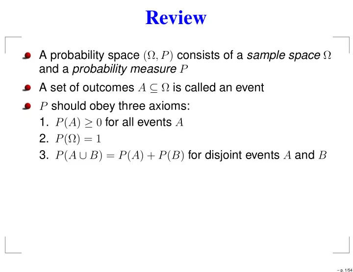
Review A probability space (Ω , P ) consists of a sample space Ω and a probability measure P A set of outcomes A ⊆ Ω is called an event P should obey three axioms: 1. P ( A ) ≥ 0 for all events A 2. P (Ω) = 1 3. P ( A ∪ B ) = P ( A ) + P ( B ) for disjoint events A and B – p. 1/54

Review A random variable X is a function from the sample space Ω to the domain dom ( X ) of X A random variable has an associated density p X : dom ( X ) → R From a joint density we can compute marginal and conditional densities The conditional probability of a A given B is P ( A | B ) = P ( A, B ) P ( B ) where P ( B ) = � a P ( a, E ) . – p. 2/54

Independence Random variable X is independent of random variable Y if for all x and y P ( x | y ) = P ( x ) This is written as X ⊥ ⊥ Y Examples: ⊥ Haircolor since P ( Flu | Haircolor ) = P ( Flu ) . Flu ⊥ ✚ ⊥ ⊥ Fever since P ( Myalgia | Fever ) � = P ( Myalgia ) . Myalgia ✚ – p. 3/54

Independence Independence is very powerful because it allows us to reason about aspects of a system in isolation. However, it does not often occur in complex systems. For example, try and think of two medical symptoms that are independent. A generalization of independence is conditional independence, where two aspects of a system become independent once we observe a third aspect. Conditional independence does often arise and can lead to significant representational and computational savings. – p. 4/54

Conditional independence Random variable X is conditionally independent of random variable Y given random variable Z if P ( x | y, z ) = P ( x | z ) whenever P ( y, z ) > 0 . That is, knowledge of Y doesn’t affect your belief in the value of X , given a value of Z . This is written as X ⊥ ⊥ Y | Z Example: Symptoms are conditionally independent given the disease: Myalgia ⊥ ⊥ Fever | Flu since P ( Myalgia | Fever , Flu ) = P ( Myalgia | Flu ) – p. 5/54

Conditional independence An intuitive test of conditional independence (Paskin): Imagine that you know the value of Z and you are trying to guess the value of X . In your pocket is an envelope containing the value of Y . Would opening the envelope help you guess X ? If not, then X ⊥ ⊥ Y | Z . – p. 6/54

Example Assume we have a joint density over the following five variables: Temperature: temp ∈ { high , low } Fever: fe ∈ { y , n } ( Myalgia: my ∈ { y , n } Flu: fl ∈ { y , n } Pneumonia: pn ∈ { y , n } Probabilistic inference amounts to computing one or more (conditional) densities given (possibly empty) observations. – p. 7/54

Conditioning and marginalization How to compute P ( pn | temp=high ) from the joint density P ( temp , fe , my , fl , pn ) ? Conditioning gives us: P ( fe , my , fl , pn | temp=high ) = P ( temp=high , fe , my , fl , pn ) P ( temp=high ) Marginalization gives us: � � P ( pn | temp=high ) = P ( fe , my , fl , pn | temp=high ) fe my 1 � � � = P ( temp=high , fe , my , fl , pn ) Z fe my fl with Z = P ( temp=high ) . – p. 8/54

Inference problem 1 � � � P ( pn | temp=high ) = P ( temp=high , fe , my , fl , pn ) Z fe my fl We don’t need to compute Z . We just compute P ( pn | temp=high ) × P ( temp=high ) and renormalize. We do need to compute the sums, which becomes expensive very fast (nested for loops)! – p. 9/54

Representation problem In order to specify the joint density P ( temp , fe , my , fl , pn ) we need to estimate 31(2 n − 1) probabilities Probabilities can be estimated by means of knowledge engineering or by parameter learning This doesn’t solve the problem How does an expert estimate P ( temp=low , fe=y , my=n , fl=y , pn=y ) ? Parameter learning requires huge databases containing multiple instances of each configuration Solution: conditional independence! – p. 10/54

Chain rule revisited The chain rule allows us to write: P ( temp , fe , my , fl , pn ) = P ( temp | fe , my , fl , pn ) P ( fe | my , fl , pn ) P ( my | fl , pn ) P ( fl | pn ) P ( pn ) This requires 16 + 8 + 4 + 2 + 1 = 31 probabilities We now make the following (conditional) independence assumptions: fl ⊥ ⊥ pn my ⊥ ⊥ { temp , fe , pn } | fl temp ⊥ ⊥ { my , fl , pn } | fe fe ⊥ ⊥ { my } | { fl , pn } – p. 11/54

Chain rule revisited By definition of conditional independence: P ( temp , fe , my , fl , pn ) = P ( temp | fe ) P ( fe | fl , pn ) P ( my | fl ) P ( fl ) P ( pn ) This requires just 2 + 4 + 2 + 1 + 1 = 10 instead of 31 probabilities Conditional independence assumptions reduce the number of required probabilities and makes the specification of the remaining probabilities easier: P ( my | fl ) : the probability of myalgia given that someone has flu P ( pn ) : the prior probability that a random person suffers from pneumonia – p. 12/54

Bayesian networks A Bayesian (belief) network is a convenient graphical representation of the independence structure of a joint density myalgia (my) ( y es/ n o) flu (fl) ( y es/ n o) fever (fe) temp ( y es/ n o) ( ≤ 37 . 5 / > 37 . 5 ) pneumonia (pn) ( y es/ n o) – p. 13/54

Bayesian networks A Bayesian network consists of: a directed acyclic graph with nodes labeled with random variables a domain for each random variable a set of (conditional) densities for each variable given its parents Bayesian networks may consist of discrete or continuous random variables, or both We focus on the discrete case A Bayesian network is a particular kind of probabilistic graphical model Many statistical methods can be represented as graphical models – p. 14/54

Specification of probabilities P ( temp , fe , my , fl , pn ) P ( my = y | fl = y ) = 0 . 96 P ( my = y | fl = n ) = 0 . 20 myalgia (my) ( y es/ n o) P ( fl = y ) = 0 . 1 P ( fe = y | fl = y, pn = y ) = 0 . 95 flu (fl) P ( fe = y | fl = n, pn = y ) = 0 . 80 ( y es/ n o) P ( fe = y | fl = y, pn = n ) = 0 . 88 P ( fe = y | fl = n, pn = n ) = 0 . 001 fever (fe) temp P ( pn = y ) = 0 . 05 ( y es/ n o) ( ≤ 37 . 5 / > 37 . 5 ) pneumonia (pn) ( y es/ n o) P ( temp ≤ 37 . 5 | fe = y ) = 0 . 1 P ( temp ≤ 37 . 5 | fe = n ) = 0 . 99 – p. 15/54

Bayesian network construction A BN can be formally constructed as follows: 1. choose an ordering of the variables; 2. apply the chain rule; and 3. use conditional independence assumptions to prune parents. The final structure depends on the variable ordering Another way to construct the network is to choose the parents of each node, and then ensure that the resulting graph is acyclic. Although BNs often model causal knowledge, they are not causal models! – p. 16/54

Bayesian network construction To represent a domain in a Bayesian network, you need to consider: What are the relevant variables? What will you observe? What would you like to find out? What other features make the model simpler? What values should these variables take? What is the relationship between them? This should be expressed in terms of local influences. How does the value of each variable depend on its parents? Expressed in terms of the conditional probabilities. – p. 17/54

Common descendants tampering and fire are independent tampering and fire are dependent given alarm tampering can explain away fire – p. 18/54

Common ancestors alarm and smoke are dependent alarm and spoke are independent given fire fire can explain alarm and smoke; learning about one can affect the other by changing your belief in fire – p. 19/54

Chain alarm and report are dependent alarm and report are independent given leaving the only way alarm affects report is by affecting leaving – p. 20/54

Testing for conditional independence Bayesian networks encode the independence properties of a joint density. If we enter evidence in a BN, the result is a conditional density that can have different independence properties. We can determine if a conditional independence X ⊥ ⊥ Y | { Z 1 , . . . , Z k } holds through the concept of d-separation X and Y are d-separated if there is no active path between them. The Bayes ball algorithm can be used to check if there are active paths – p. 21/54

The Bayes ball algorithm – p. 22/54

Example – p. 23/54

Inference: evidence propagation Nothing known: MYALGIA NO YES FLU NO YES FEVER TEMP NO <=37.5 YES >37.5 PNEUMONIA NO YES Which symptoms belong to flu? MYALGIA NO YES FLU NO YES FEVER TEMP NO <=37.5 YES >37.5 PNEUMONIA NO YES – p. 24/54

Inference: evidence propagation Nothing known: MYALGIA NO YES FLU NO YES FEVER TEMP NO <=37.5 YES >37.5 PNEUMONIA NO YES Temperature > 37 . 5 grades Celcius: MYALGIA NO YES FLU NO YES FEVER TEMP NO <=37.5 YES >37.5 PNEUMONIA NO YES – p. 25/54

Efficient inference Conditional independence assumptions not only solve the representation problem but also make inference easier By plugging in the factorized density we obtain: P ( pn | temp=high ) � � � ∝ P ( temp=high , fe , my , fl , pn ) fe my fl � � � = P ( temp=high | fe ) P ( fe | fl , pn ) P ( my | fl ) P ( fl ) P ( pn ) fe my fl Inference reduces to computing sums of products. An efficient way to do this is using variable elimination – p. 26/54

Variable elimination How can we compute ab + ac efficiently? – p. 27/54

Variable elimination How can we compute ab + ac efficiently? Distribute out a giving a ( b + c ) → 2 instead of 3 elementary operations – p. 27/54