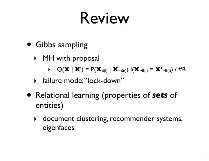
Review Gibbs sampling MH with proposal Q( X | X ) = P( X B(i) | X - PowerPoint PPT Presentation

Review • Gibbs sampling ‣ MH with proposal ‣ Q( X | X ’) = P( X B(i) | X ¬B(i) ) I( X ¬B(i) = X’ ¬B(i) ) / #B ‣ failure mode: “lock-down” • Relational learning (properties of sets of entities) ‣ document clustering, recommender systems, eigenfaces 1

Review • Latent-variable models • PCA, pPCA, Bayesian PCA ‣ everything Gaussian ‣ E(X | U,V) = UV T ‣ MLE: use SVD • Mean subtraction, example weights 2

PageRank • SVD is pretty useful: turns out to be main computational step in other models too • A famous one: PageRank ‣ Given: web graph (V, E) ‣ Predict: which pages are important 3

PageRank: adjacency matrix 4

Random surfer model ‣ W. p. α : ‣ W. p. (1– α ): ‣ Intuition: page is important if a random surfer is likely to land there 5

Stationary distribution 0.5 0.4 0.3 0.2 0.1 0 A B C D 6

Thought experiment • What if A is symmetric? ‣ note: we’re going to stop distinguishing A, A’ • So, stationary dist’n for symmetric A is: • What do people do instead? 7

Spectral embedding • Another famous model: spectral embedding (and its cousin, spectral clustering) • Embedding: assign low-D coordinates to vertices (e.g., web pages) so that similar nodes in graph ⇒ nearby coordinates ‣ A, B similar = random surfer tends to reach the same places when starting from A or B 8

Where does random surfer reach? • Given graph: • Start from distribution π ‣ after 1 step: P(k | π , 1-step) = ‣ after 2 steps: P(k | π , 2-step) = ‣ after t steps: 9

Similarity • A, B similar = random surfer tends to reach the same places when starting from A or B • P(k | π , t-step) = ‣ If π has all mass on i: ‣ Compare i & j: ‣ Role of Σ t : 10

Role of Σ t (real data) 1 t=1 t=3 t=5 0.8 t=10 0.6 0.4 0.2 0 2 4 6 8 10 11

Example: dolphins 0 10 20 30 40 50 (Lusseau et al., 2003) 60 0 20 40 60 • 62-dolphin social network near Doubtful Sound, New Zealand ‣ A ij = 1 if dolphin i friends dolphin j 12

Dolphin network !"% !"# !"$ ! ! !"$ ! !"# ! !"% ! !"# ! !"$ ! !"$ !"# !"% 13

Comparisons !"# !"& !"% !"# !"$ !"$ !"& !"% ! ! ! !"& ! !"% ! !"$ ! !"$ ! !"% ! !"# ! !"# ! !"# ! !"$ ! !"$ !"# ! !"# ! !"$ ! !"% ! !"% !"$ !"# spectral embedding of random embedding of random data dolphin data 14

Spectral clustering !"% !"# !"$ ! ! !"$ ! !"# ! !"% ! !"# ! !"$ ! !"$ !"# !"% • Use your favorite clustering algorithm on coordinates from spectral embedding 15

PCA: the good, the bad, and the ugly • The good: simple, successful • The bad: linear, Gaussian ‣ E(X) = UV T ‣ X, U, V ~ Gaussian • The ugly: failure to generalize to new entities 16

Consistency • Linear & logistic regression are consistent • What would consistency mean for PCA? ‣ forget about row/col means for now • Consistency: ‣ #users, #movies, #ratings (= nnz(W)) ‣ numel(U), numel(V) ‣ consistency = 17

Failure to generalize • What does this mean for generalization? ‣ new user’s rating of movie j : only info is ‣ new movie rated by user i : only info is ‣ all our carefully-learned factors give us: • Generalization is: 18

Hierarchical model old, non-hierarchical model 19

Benefit of hierarchy • Now: only k μ U latents, k μ V latents (and corresponding σ s) ‣ can get consistency for these if we observe more and more X ij • For a new user or movie: 20

Mean subtraction • Can now see that mean subtraction is a special case of our hierarchical model ‣ Fix V j1 = 1 for all j; then U i1 = ‣ Fix U i2 = 1 for all i; then V j2 = ‣ global mean: 21

What about the second rating for a new user? • Estimating U i from one rating: ‣ knowing μ U : ‣ result: • How should we fix? • Note: often we have only a few ratings per user 22

MCMC for PCA • Can do Bayesian inference by Gibbs sampling—for simplicity, assume σ s known 23

Recognizing a Gaussian • Suppose X ~ N(X | μ , σ 2 ) • L = –log P(X=x | μ , σ 2 ) = ‣ dL/dx = ‣ d 2 L/dx 2 = • So: if we see d 2 L/dx 2 = a, dL/dx = a(x – b) ‣ μ = σ 2 = 24

Gibbs step for an element of μ U 25

Gibbs step for an element of U 26

In reality • We’d do blocked Gibbs instead • Blocks contain entire rows of U or V ‣ take gradient, Hessian to get mean, covariance ‣ formulas look a lot like linear regression (normal equations) • And, we’d fit σ U , σ V too ‣ sample 1/ σ 2 from a Gamma (or Σ –1 from a Wishart ) distribution 27

Nonlinearity: conjunctive features P(rent) Foreign Comedy 28

Disjunctive features P(rent) Comedy Foreign 29

“Other” P(rent) Comedy Foreign 30

Non-Gaussian • X, U, and V could each be non-Gaussian ‣ e.g., binary! ‣ rents(U, M), comedy(M), female(U) • For X: predicting –0.1 instead of 0 is only as bad as predicting +0.1 instead of 0 • For U, V: might infer –17% comedy or 32% female 31

Logistic PCA • Regular PCA: X ij ~ N(U i ⋅ V j , σ 2 ) • Logistic PCA: 32

More generally… • Can have ‣ X ij ∼ Poisson( μ ij ), μ ij = exp(U i ⋅ V j ) ‣ X ij ∼ Bernoulli( μ ij ), μ ij = σ (U i ⋅ V j ) ‣ … • Called exponential family PCA • Might expect optimization to be difficult 33

Application: fMRI Brain activity fMRI :-) stimulus: “dog” fMRI ;-> stimulus: “cat” fMRI stimulus: “hammer” :-)) credit: Ajit Singh Voxels Stimulus Y 34

Results (logistic PCA) Y (fMRI data): Fold-in 1.4 HB � CMF H � CMF Maximum a posteriori (fixed hyperparameters) 1.2 CMF 1 Mean Squared Error 0.8 Lower is credit: Ajit Singh 0.6 0.4 Better 0.2 0 Augmenting fMRI data with Just using fMRI data word co-occurrence 35