Resource-aware Program Analysis via Online Abstraction Coarsening - PowerPoint PPT Presentation
Resource-aware Program Analysis via Online Abstraction Coarsening Kihong Heo Hakjoo Oh Hongseok Yang ICSE 2019 1 Motivation Deep semantic analysis for large software 30M 25M 20M Size (LOC) 15M 10M 5M 0M 1.0 2.0 2.6.16
Resource-aware Program Analysis via Online Abstraction Coarsening Kihong Heo Hakjoo Oh Hongseok Yang ICSE 2019 � 1
Motivation • Deep semantic analysis for large software 30M 25M 20M Size (LOC) 15M 10M 5M 0M 1.0 2.0 2.6.16 2.6.34 3.10 4.1 4.19 X (1st LTS) (5th LTS) (10th LTS) (15th LTS) (19th LTS) Linux Kernel Version *https://www.linuxcounter.net � 2
Motivation • Deep semantic analysis for large software 30M 25M 20M Size (LOC) 15M 10M 5M 0M 1.0 2.0 2.6.16 2.6.34 3.10 4.1 4.19 X (1st LTS) (5th LTS) (10th LTS) (15th LTS) (19th LTS) Linux Kernel Version *https://www.linuxcounter.net � 2
Motivation • Deep semantic analysis for large software ! 30M 25M 20M Size (LOC) 15M 10M 5M 0M 1.0 2.0 2.6.16 2.6.34 3.10 4.1 4.19 X (1st LTS) (5th LTS) (10th LTS) (15th LTS) (19th LTS) Linux Kernel Version *https://www.linuxcounter.net � 2
Goal � 3
Goal • Achieving maximum precision within a given resource budget • e.g., within 128GB of memory � 3
Goal • Achieving maximum precision within a given resource budget • e.g., within 128GB of memory X-sensitivity (knob) � 4
Goal • Achieving maximum precision within a given resource budget • e.g., within 128GB of memory Low Precision Low Utilization X-sensitivity (knob) � 4
Goal • Achieving maximum precision within a given resource budget • e.g., within 128GB of memory Out of Resource X-sensitivity (knob) � 4
Goal • Achieving maximum precision within a given resource budget • e.g., within 128GB of memory Max. Precision Max. Utilization X-sensitivity (knob) � 4
Challenges • Hard to predict the behavior of analyzer in advance • e.g., partially flow-sensitive interval analysis � 5
Challenges • Hard to predict the behavior of analyzer in advance • e.g., partially flow-sensitive interval analysis Sensitivity: 0% emacs-26.0.91 (503KLOC) Memory: 18GB � 5
Challenges • Hard to predict the behavior of analyzer in advance • e.g., partially flow-sensitive interval analysis Sensitivity: 0% Sensitivity: 5% < emacs-26.0.91 emacs-26.0.91 (503KLOC) (503KLOC) Memory: 18GB � 5
Challenges • Hard to predict the behavior of analyzer in advance • e.g., partially flow-sensitive interval analysis Sensitivity: 0% Sensitivity: 5% < emacs-26.0.91 emacs-26.0.91 (503KLOC) (503KLOC) << Memory: Memory: 18GB > 128GB � 5
Challenges • Hard to predict the behavior of analyzer in advance • e.g., partially flow-sensitive interval analysis Sensitivity: 0% Sensitivity: 0% Sensitivity: 5% < < vim60 emacs-26.0.91 emacs-26.0.91 (227KLOC) (503KLOC) (503KLOC) << Memory: Memory: 18GB > 128GB � 5
Challenges • Hard to predict the behavior of analyzer in advance • e.g., partially flow-sensitive interval analysis Sensitivity: 0% Sensitivity: 0% Sensitivity: 5% < < vim60 emacs-26.0.91 emacs-26.0.91 (227KLOC) (503KLOC) (503KLOC) > << Memory: Memory: Memory: 18GB > 128GB 51GB � 5
Our Approach • Online abstraction coarsening by a learned controller Budget Resource Precision Usage Analysis Progress � 6
Our Approach • Online abstraction coarsening by a learned controller Budget Resource Precision Usage Low-sensitivity Analysis Progress � 6
Our Approach • Online abstraction coarsening by a learned controller High-sensitivity Budget Resource Precision Usage Low-sensitivity Analysis Progress � 6
Our Approach • Online abstraction coarsening by a learned controller High-sensitivity Our approach Budget Resource Precision Usage Low-sensitivity Analysis Progress � 6
Our Approach • Online abstraction coarsening by a learned controller High-sensitivity Our approach Budget O ffl ine Approach Online Approach (10% flow-sensitivity) Resource Precision Usage Low-sensitivity Analysis Progress � 7
Our Approach • Online abstraction coarsening by a learned controller High-sensitivity Our approach Budget O ffl ine Approach Online Approach (10% flow-sensitivity) Resource • 3/8 run out of memory (128GB) Precision Usage • 27% of bu ff er overrun alarms � • 30% of null dereference alarms � Low-sensitivity Analysis Progress � 7
Our Approach • Online abstraction coarsening by a learned controller High-sensitivity Our approach Budget O ffl ine Approach Online Approach (10% flow-sensitivity) Resource • 0/8 run out of memory (64 / 128GB) • 3/8 run out of memory (128GB) Precision Usage • 28—32% of bu ff er overrun alarms � • 27% of bu ff er overrun alarms � • 30% of null dereference alarms � • 33—41% of null dereference alarms � Low-sensitivity Analysis Progress � 7
Outline • Motivation • Learning Framework • Experimental Results • Conclusion � 8
Example • Partially flow-sensitive interval analysis (budget: 10 intervals) 1: x = 0; y = 0; z = 1; v = input(); w = input(); 2: x = z; 3: z = z + 1; 4: y = x; 5: assert(y > 0); // Query 1 (hold) 6: assert(z > 0); // Query 2 (hold) 7: assert(v == w); // Query 3 (may fail) � 9
Example • Partially flow-sensitive interval analysis (budget: 10 intervals) 1: x = 0; y = 0; z = 1; v = input(); w = input(); 2: x = z; 3: z = z + 1; 4: y = x; 5: assert(y > 0); // Query 1 (hold) 6: assert(z > 0); // Query 2 (hold) 7: assert(v == w); // Query 3 (may fail) Line Flow-Sensitive Abstract State 1 {x = [0,0], y = [0,0], z = [1,1], v = ⊤ , w = ⊤ } 2 {x = [1,1], y = [0,0], z = [1,1], v = ⊤ , w = ⊤ } 3 Intervals 12 Intervals 3 {x = [1,1], y = [0,0], z = [2,2], v = ⊤ , w = ⊤ } 4 {x = [1,1], y = [1,1], z = [2,2], v = ⊤ , w = ⊤ } � 10
Example • Partially flow-sensitive interval analysis (budget: 10 intervals) 1: x = 0; y = 0; z = 1; v = input(); w = input(); 2: x = z; 3: z = z + 1; 4: y = x; 5: assert(y > 0); // Query 1 (hold) 6: assert(z > 0); // Query 2 (hold) 7: assert(v == w); // Query 3 (may fail) Line Flow-Sensitive Abstract State 1 {x = [0,0], y = [0,0], z = [1,1], v = ⊤ , w = ⊤ } 2 {x = [1,1], y = [0,0], z = [1,1], v = ⊤ , w = ⊤ } 3 {x = [1,1], y = [0,0], z = [2,2], v = ⊤ , w = ⊤ } 6 Intervals 4 {x = [1,1], y = [1,1], z = [2,2], v = ⊤ , w = ⊤ } � 11
Example • Partially flow-sensitive interval analysis (budget: 10 intervals) 1: x = 0; y = 0; z = 1; v = input(); w = input(); 2: x = z; 3: z = z + 1; 4: y = x; 5: assert(y > 0); // Query 1 (hold) 6: assert(z > 0); // Query 2 (hold) 7: assert(v == w); // Query 3 (may fail) Line Flow-Sensitive Abstract State 1 {x = [0,0], y = [0,0], z = [1,1], v = ⊤ , w = ⊤ } 2 {x = [1,1], y = [0,0], z = [1,1], v = ⊤ , w = ⊤ } 3 {x = [1,1], y = [0,0], z = [2,2], v = ⊤ , w = ⊤ } { x = [1,1], y = [1,1], z = [2,2] , v = ⊤ , w = ⊤ } 4 12 Intervals � 12
Example • Partially flow-sensitive interval analysis (budget: 10 intervals) 1: x = 0; y = 0; z = 1; v = input(); w = input(); 2: x = z; 3: z = z + 1; 4: y = x; 5: assert(y > 0); // Query 1 (hold) 6: assert(z > 0); // Query 2 (hold) 7: assert(v == w); // Query 3 (may fail) Line Flow-Insensitive Abstract State { x = [0,+ ∞ ], y = [0,+ ∞ ], z = [1,+ ∞ ] , v = ⊤ , w = ⊤ } * 3 Intervals � 13
Online Abstraction Coarsening � 14
Online Abstraction Coarsening Analyzer Input Result � 14
Online Abstraction Coarsening Analyzer M 0 Transfer Input Result Function � 14
Online Abstraction Coarsening Analyzer M 0 M i Transfer Input Result Fixpoint? Function � 14
Online Abstraction Coarsening Analyzer M 0 M i Y Transfer Input Result Fixpoint? Function � 14
Online Abstraction Coarsening Analyzer M 0 M i Y Transfer Input Result Fixpoint? Function N M i Controller Model � 14
Online Abstraction Coarsening Analyzer M 0 M i Y Transfer Input Result Fixpoint? Function N M i+1 M i Controller Model � 14
Model � 15
Model • Model M : Variable → [0, 1] • Importance of each variable in terms of flow-sensitivity • Pre-trained by an o ff -the-shelf method* *Learning a Strategy for Adapting a Program Analysis via Bayesian Optimisation, OOPSLA’15 � 15
Model • Model M : Variable → [0, 1] • Importance of each variable in terms of flow-sensitivity • Pre-trained by an o ff -the-shelf method* 1: x = 0; y = 0; z = 1; v = input(); w = input(); 2: x = z; 3: z = z + 1; 4: y = x; 5: assert(y > 0); // Query 1 (hold) 6: assert(z > 0); // Query 2 (hold) 7: assert(v == w); // Query 3 (may fail) *Learning a Strategy for Adapting a Program Analysis via Bayesian Optimisation, OOPSLA’15 � 15
Model • Model M : Variable → [0, 1] • Importance of each variable in terms of flow-sensitivity • Pre-trained by an o ff -the-shelf method* 1: x = 0; y = 0; z = 1; v = input(); w = input(); 2: x = z; 3: z = z + 1; 4: y = x; 5: assert(y > 0); // Query 1 (hold) 6: assert(z > 0); // Query 2 (hold) 7: assert(v == w); // Query 3 (may fail) > M(w) *Learning a Strategy for Adapting a Program Analysis via Bayesian Optimisation, OOPSLA’15 � 15
Recommend
More recommend
Explore More Topics
Stay informed with curated content and fresh updates.

