RELATIVE AND ABSOLUTE EXTREMA MATH 200 GOALS Be able to use - PowerPoint PPT Presentation

MATH 200 WEEK 6 - FRIDAY RELATIVE AND ABSOLUTE EXTREMA

MATH 200 GOALS ▸ Be able to use partial derivatives to find critical points (possible locations of maxima or minima). ▸ Know how to use the Second Partials Test for functions of two variables to determine whether a critical point is a relative maximum , relative minimum , or a saddle point . ▸ Be able to solve word problems involving maxima and minima. ▸ Know how to compute absolute maxima and minima on closed regions.

MATH 200 FROM CALC 1 ▸ Given a function f(x), how do we find its relative extrema ? ▸ Find the critical points: ▸ f’(x) = 0 ▸ f’ is undefined ▸ Do either the first or second derivative test ▸ First derivative test: make a sign chart for f’ ▸ Second derivative test: look at the concavity of f at each critical point

MATH 200 ▸ Example: Second Derivative Test ▸ Consider the function f(x) = x 4 - 2x 2 Relative Maximum at x = 0 ▸ f’(x) = 4x 3 - 4x = 4x(x 2 - 1) ▸ Critical points: x=-1,0,1 (because f’(-1)=0, f’(0)=0, f’(1)=0) ▸ f’’(x) = 12x 2 - 4 ▸ f’’(-1) = 8 > 0 so f is concave up at x=-1 ▸ f’’(0) = -4 < 0 so f is concave Relative Minima at x = -1 down at x=0 and x = 1 ▸ f’’(1) = 8 > 0 so f is concave up at x=1

MATH 200 NEW STUFF ▸ The process for finding relative (local) extrema for functions of three variables follows the second derivative test from calc 1 pretty closely…but has a few more moving parts ▸ Step 1: Find critical points ▸ Places where we might have a relative extremum ▸ Step 2: Test the concavity of the function at the critical points ▸ If f is concave up at a critical point, it’s a relative min ▸ If f is concave down at a critical point, it’s a relative max

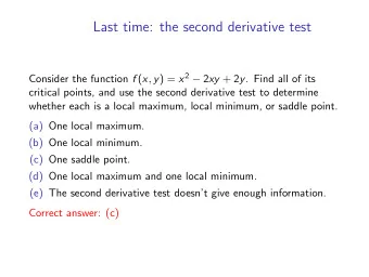
MATH 200 ▸ Critical Points: We say that (x 0 ,y 0 ) is a critical point for f provided that f x (x 0 ,y 0 ) = 0 and f y (x 0 ,y 0 ) = 0 ▸ Define D = f xx f yy - (f xy ) 2 ▸ If D(x 0 ,y 0 ) > 0 and f xx (x 0 ,y 0 ) < 0 , then f has a relative maximum at (x 0 ,y 0 ) ▸ If D(x 0 ,y 0 ) > 0 and f xx (x 0 ,y 0 ) > 0 , then f has a relative minimum at (x 0 ,y 0 ) ▸ If D(x 0 ,y 0 ) < 0 , then f has a saddle point at (x 0 ,y 0 ) ▸ If D(x 0 ,y 0 ) = 0, then the test fails…

MATH 200 AN EASY EXAMPLE (WE ALREADY KNOW THE ANSWER) ▸ Consider the paraboloid f(x,y) = x 2 + y 2 ▸ We already know (hopefully) that f has a relative minimum at (0,0), but let’s show this using the second derivative test. ▸ Find the critical points: � � � f x ( x, y ) = 2 x 2 x = 0 x = 0 = = ⇒ ⇒ f y ( x, y ) = 2 y 2 y = 0 y = 0 ▸ So, we have one critical point: (0,0)

MATH 200 ▸ Test the concavity of f at (0,0) by looking at D: D ( x, y ) = f xx ( x, y ) f yy ( x, y ) − ( f xy ( x, y )) 2 ▸ To do so we need the second order partial derivatives: f xx ( x, y ) = 2; f yy ( x, y ) = 2; f xy ( x.y ) = 0 ▸ Since these are all constant, the calculation is pretty easy: D(0,0) = (2)(2) - 0 = 4 > 0 ▸ Since D(0,0) > 0 and f xx (0,0) > 0 we have a relative minimum at (0,0)

MATH 200

MATH 200 EXAMPLE 1 ▸ Consider the function f ( x, y ) = x 2 y 3 − 3 2 y 2 − x 2 ▸ Find the critical points by setting f x and f y equal to zero � � f x ( x, y ) = 2 xy 3 − 2 x 2 xy 3 − 2 x = 0 f y ( x, y ) = 3 x 2 y 2 − 3 y 3 x 2 y 2 − 3 y = 0 ▸ In the first equation, we can factor out a 2x 2 x ( y 3 − 1) = 0 = ⇒ x = 0 , y = 1 THIS DOES NOT MEAN (0,1) IS A CRITICAL POINT! WE CAN TELL BECAUSE IT DOESN’T WORK IN THE Y-DERIVATIVE

MATH 200 ▸ x = 0 makes the x-partial zero for any y-value. Let’s plug that into the y-partial and see what happens 3 x 2 y 2 − 3 y = 0 = ⇒ 3(0) 2 y 2 − 3 y = 0 − 3 y = 0 y = 0 ▸ That’s one critical point: (0,0) ▸ Let’s do the same for y = 1: 3 x 2 y 2 − 3 y = 0 = ⇒ 3 x 2 (1) 2 − 3(1) = 0 3 x 2 − 3 = 0 x 2 − 1 = 0 x = ± 1 ▸ That’s two more critical points: (-1,1) and (1,1)

MATH 200 ▸ So far, we’ve found that f has three critical points. Now we want to test the concavity of f using D. D ( x, y ) = f xx ( x, y ) f yy ( x, y ) − ( f xy ( x, y )) 2 f xx = 2 y 3 − 2; f yy = 6 x 2 y − 3; f xy = 6 xy 2 If D(x 0 ,y 0 ) > 0 and f xx (x 0 ,y 0 ) < 0 , then f has a relative maximum at (x 0 ,y 0 ) If D(x 0 ,y 0 ) > 0 and f xx (x 0 ,y 0 ) > 0 , then f has a relative minimum at (x 0 ,y 0 ) If D(x 0 ,y 0 ) < 0 , then f has a saddle point at (x 0 ,y 0 ) (x,y) f xx (x,y) f yy (x,y) f xy (x,y) D(x,y) Type (0,0) -2 -3 0 6 Relative Max Saddle Point (-1,1) 0 3 -6 -36 Saddle Point (1,1) 0 3 6 -36

MATH 200 RELATIVE MAXIMUM SADDLE POINTS

MATH 200 EXAMPLE 2 ▸ Find all relative extrema for f(x,y) = 4 + x 3 + y 3 - 3xy � � f x ( x, y ) = 3 x 2 − 3 y 3 x 2 − 3 y = 0 = ⇒ f y ( x, y ) = 3 y 2 − 3 x 3 y 2 − 3 x = 0 ▸ We have to be a little more clever here…solve the x-partial for y: 3 y = 3 x 2 = ⇒ y = x 2 ▸ Now plug that into the y-partial 3( x 2 ) 2 − 3 x = 0 3 x 4 − 3 x = 0 3 x ( x 3 − 1) = 0 x = 0 , 1

MATH 200 ▸ Now we put together what we know: f xx ( x, y ) = 6 x ▸ y = x 2 and x = 0 or 1 f yy ( x, y ) = 6 y f xy ( x, y ) = − 3 ▸ y = (0) 2 = 0 ▸ y = (1) 2 = 1 D = f xx f yy − ( f xy ) 2 ▸ Critical Points: (0,0), (1,1) (x,y) f xx f yy f xy D Type ▸ Finally, we test the concavity of f at these (0,0) 0 0 -3 -9 Saddle points using D (1,1) 6 6 -3 27 Rel. Min

MATH 200 SADDLE POINT RELATIVE MINIMUM

MATH 200 ABSOLUTE EXTREMA ON A CLOSED INTERVAL (FROM CALC 1) ▸ Extreme value theorem : If a function f(x) is continuous on a closed interval [a,b], then f is guaranteed to have both a maximum value and a minimum value on [a,b] ▸ How we use the EVT for a continuous f on [a,b]: ▸ Find critical points on [a,b] ▸ Evaluate f(x) at each critical point inside [a,b] as well as at the endpoints (i.e. f(a) and f(b)) ▸ Compare f-values and identify maximum and minimum

MATH 200 ▸ A quick Calc 1 example: f(x) = x 3 - 6x 2 + 3 on [-1,5] ▸ First we find the critical points ▸ f’(x) = 3x 2 - 12x = 3x(x-4) ▸ Critical points: x = 0, 4 ▸ Evaluate f at x = -1, 0, 4, 5 ▸ f(-1) = -5 ▸ f(0) =3 ABSOLUTE MAX: 3 AT X = 0 ▸ f(4) = -29 ABSOLUTE MIN: -29 AT X = 4 ▸ f(5) = -22

MATH 200 NEW STUFF: CLOSED REGIONS ▸ For functions of two variables, we need to talk about closed and bounded regions rather than closed intervals ▸ Compare closed regions and open intervals 3 x 4 + 4 x 2 y + y 4 ≤ 4 3 x 4 + 4 x 2 y + y 4 < 4

MATH 200 UPDATED EXTREME VALUE THEOREM ▸ If f(x,y) is continuous on a closed and bounded region R, then it must attain both a maximum value and a minimum value on that region. ▸ How to apply the EVT: ▸ Find all critical points for f inside the region R ▸ Restrict f to the boundary of R ▸ Apply the single-variable EVT to f restricted to the boundary ▸ Compare the values of f at the critical points inside R with the absolute extrema on the boundary

MATH 200 EXAMPLE ▸ Consider f(x,y) = x 2 + y 2 ▸ We want to restrict f to the restricted to the elliptic region boundary of R R: x 2 + 4y 2 ≤ 4 ▸ Boundary: x 2 + 4y 2 = 4 ▸ First we find the critical points for f inside R ▸ x 2 = 4 - 4y 2 ▸ f x = 2x ▸ Replacing x 2 with 4 - 4y 2 we get a function of y ▸ f y = 2y ▸ Critical point: (0,0) ▸ b(y) = 4 - 4y 2 + y 2 ▸ It’s certainly in R since 0 2 ▸ b(y) = 4 - 3y 2 + 4(0) 2 = 0 ≤ 4

MATH 200 ▸ Now we can apply the EVT to b(y) ▸ Compare these values with what we get for f at the critical point (0,0) on the interval [-1,1] ▸ f(0,0) = 0 ▸ Why [-1,1]? Because the ellipse extends from y=-1 to y=1. ▸ So the absolute minimum is 0, which occurs at (0,0) ▸ b(y) = 4 - 3y 2 ▸ The absolute maximum is 4 which ▸ Find critical points: b’(y) = -6y occurs on the boundary of R when y=0 ▸ y = 0 ▸ What is x when y=0 on the ▸ Evaluate and compare: boundary? ▸ b(0) = 4 ▸ x 2 = 4 - 4y 2 ▸ b(-1) = 1 ▸ x = -2 or 2 ▸ So, the absolute maximum occurs at ▸ b(1) = 1 (-2,0) and (2,0)

MATH 200

MATH 200 ANOTHER EXAMPLE ▸ Find the absolute extrema for f(x,y) = x 2 + 4y 2 - 2x 2 y + 4 on the square S = {(x,y):-1 ≤ x ≤ 1 and -1 ≤ y ≤ 1} ▸ First, we’ll find the critical points in R � � f x ( x, y ) = 2 x − 4 xy 2 x − 4 xy = 0 8 y − 2 x 2 = 0 f y ( x, y ) = 8 y − 2 x 2 ▸ Factor 2x in the x-partial: 2 x (1 − 2 y ) = 0 = ⇒ x = 0 , y = 1 / 2 ▸ Now we plug x=0 and y=1/2 into the y-partial y = 1 / 2 : 4 − 2 x 2 = 0 x = 0 : 8 y = 0 √ y = 0 x = ± 2

f(x,y) = x 2 + 4y 2 - 2x 2 y + 4 MATH 200 √ √ ▸ f has three critical points: (0 , 0) , ( 2 , 1 / 2) , ( − 2 , 1 / 2) ▸ But only (0,0) is in S! ▸ Evaluate: f(0,0) = 4 ▸ Now we need to see what happens on the boundary . ▸ S is a square, so we have to look at each side separately ▸ Bottom of square: y=-1 and -1 ≤ x ≤ 1 ▸ To restrict f to this boundary piece, we set y=-1 ▸ b(x) = f(x,-1) = x 2 + 4(-1) 2 - 2x 2 (-1) + 4 = 3x 2 + 8 ▸ b’(x) = 6x ▸ Critical point: x = 0 ▸ b(0) = f(0,-1) = 8

f(x,y) = x 2 + 4y 2 - 2x 2 y + 4 MATH 200 ▸ Top: y = 1 and -1 ≤ x ≤ 1 ▸ Restrict f: b(x) = f(x,1) = x 2 + 4(1) 2 - 2x 2 (1) + 4 = 8 - x 2 ▸ b’(x) = -2x ▸ Critical point: x = 0 ▸ b(0) = f(0,1) = 8 ▸ Left: x = -1 and -1 ≤ y ≤ 1 ▸ Restrict f: b(y) = f(-1,y) = (-1) 2 + 4y 2 - 2(-1) 2 y + 4 = 4y 2 - 2y + 5 ▸ b’(y) = 8y - 2 ▸ Critical point: y = 1/4 ▸ b(1/4) = f(-1,1/4) = 19/4