Related to Bayesian Statistics by Atsuhide Mori (Osaka Dental - PowerPoint PPT Presentation
Symplectic/Contact Geometry Related to Bayesian Statistics by Atsuhide Mori (Osaka Dental University, Japan) Geometric setting (1) The mind and statistics : manifold that stands for (a part of) the mind of an agent. Each point of
Symplectic/Contact Geometry Related to Bayesian Statistics by Atsuhide Mori (Osaka Dental University, Japan)
Geometric setting (1) The mind and statistics • ℳ : manifold that stands for (a part of) the mind of an agent. • Each point of ℳ presents a probability density function on ℝ 𝑜 . • Fix the state 𝑊 ∈ 𝒲 = volume forms with finite total on ℳ of ℳ . Then any statistic 𝑔: ℳ → ℝ 𝑛 obeys a probability distribution. ℝ 𝑛 ℳ 𝑔 ℝ 𝑜 (∋ 𝑨) 𝑊 /𝑒Vol =density w/ probability 𝑧 𝑔 𝑧 The proportion in ℳ by volume defines the probability . This probability distribution is the FULL estimation of the statistic 𝑔 . (A value and a confidence interval with error bar are not enough!)
Geometric setting (2) Bayesian updating • Given a point 𝑨 ∈ ℝ 𝑜 , the agent updates 𝑊 ∈ 𝒲 in the following way: Each point 𝑧 of the mind ℳ presents a probability density 𝜍 𝑧 of ℝ 𝑜 . Change it to the likelihood 𝜍 𝑨 𝑧 = 𝜍 𝑧 (𝑨) , and define the map 𝜒: ℝ 𝑜 × 𝒲 ∋ 𝑨, 𝑊 ↦ 𝜍 𝑨 𝑊 ∈ 𝒲 : “ updating map ” . • Example. ℳ = N 𝜈, 𝛵 | 𝜈 ∈ ℝ 𝑜 𝑔 = 𝜈: ℳ → ℝ 𝑜 . 𝛵 ∈ 𝒬 𝑜 , This is the estimation of the mean 𝜈 of a normal distribution with a fixed covariance 𝛵 in the space 𝒬 𝑜 of positive definite real symmetric matrix. Then the updating map is 𝜒 𝑨, 𝑊 = N 𝑨, 𝛵 𝑊 ∈ 𝒲 , namely, 𝑊 ↦ N 𝑨 1 , 𝛵 𝑊 ↦ N 𝑨 2 , 𝛵 N 𝑨 1 , 𝛵 𝑊 ↦ ⋯ . (The symmetry N 𝜈, 𝛵 𝑨 = N 𝑨, 𝛵 𝜈 implies 𝜍 𝑨 = N(𝑨, 𝛵) .)
Geometric setting (3) Conjugate prior • Our subject is the updating map 𝜒: ℝ 𝑜 × 𝒲 ∋ 𝑨, 𝑊 ↦ 𝜍 𝑨 𝑊 ∈ 𝒲 . 𝒱 ⊂ 𝒲 with 𝜒 ℝ 𝑜 × ෨ • Conjugate prior is a proper subset ෨ 𝒱 ⊂ ෨ 𝒱 . Putting 𝒱 = 𝑊 ∈ ෨ ℳ 𝑊 = 1 , we have ෨ 𝒱 | 𝒱 = 𝑙𝑊 | 𝑊 ∈ 𝒱, 𝑙 > 0 . • Example. ℳ = N 𝜈, 𝛵 | 𝜈 ∈ ℝ 𝑜 𝑜 , 𝑔 = 𝜈: ℳ → ℝ 𝑜 . Put 𝛵 ∈ 𝒬 ⇒ ෨ 𝒱 = N 𝑛, 𝐵 𝑒Vol | 𝑛 ∈ ℝ 𝑜 , 𝐵 ∈ 𝒬 𝑜, ℝ 𝒱: conjugate prior. • Suppose that the conjugate prior ෨ 𝒱 is a manifold. We fix a ``distance’’ 𝐸: ෨ ෩ 𝒱 × ෨ 𝒱 → ℝ , which satisfies non of the axioms of distance, as 1 ln 𝑊 2 ෩ 2 = න 𝐸 𝑊 1 , 𝑊 ℝ 𝑜 𝑊 the relative entropy 𝑊 1 • The restriction ෩ 𝐸| 𝒱×𝒱 = 𝐸 is non-negative ( KL-divergence ).
Geometric setting (4) Bayesian Information Geom. • Each 𝑧 ∈ ℳ presents a volume form 𝜍 𝑧 𝑒Vol on ℝ 𝑜 ∋ 𝑨 . • Given points 𝑨 1 , 𝑨 2 , … ∈ ℝ 𝑜 , one updates the prior 𝑄 ∈ ෨ 𝒱 as 𝑄 ↦ 𝜍 𝑨 1 𝑄 ↦ 𝜍 𝑨 2 𝜍 𝑨 1 𝑄 ↦ ⋯ 𝜍(𝑨)(𝑧) = 𝜍 𝑧 (𝑨) . This corresponds to a point move on 𝒱 by normalizing the density. • Generalized IG = the Fisher metric & 𝛽 -connections 𝛼 − 𝛽 ∗ 𝑈 : the quadratic term of ෩ 𝐸 𝑄, 𝑄 + 𝑒𝑄 + ෩ 𝐸(𝑄 + 𝑒𝑄, 𝑄) 𝑈 : the cubic term of 3෩ 𝐸 𝑄, 𝑄 + 𝑒𝑄 − 3෩ 𝐸 𝑄 + 𝑒𝑄, 𝑄 The usual IG looks at the restrictions to the hypersurface 𝒱 . Bayesian IG is the geometric study on the updating maps in ෨ 𝒱 and 𝒱 .
Example of Bayesian IG (1) Two operations 1 2 𝑨 − 𝜈 T 𝛵 −1 (𝑨 − 𝜈) 𝑒Vol on ℝ 𝑜 (∋ 𝑨) . • 𝜈 = 𝑧 presents exp − and ෨ • We have 𝒱 = N 𝑛, 𝐵 𝑒Vol | 𝑛 ∈ ℝ 𝑜 , 𝐵 ∈ 𝒬 𝑜, ℝ 𝒱 . 2𝑤 𝜈 2 𝑒Vol ∈ ෨ 1 • If 𝑨 repeats, the agent updates e.g. exp − 𝒱 into 𝜍 𝑨 𝑜 𝑊 = exp − 1 2𝑤 𝜈 2 − 𝑜 2 𝜈 − 𝑧 T 𝛵 −1 (𝜈 − 𝑧) 𝑒Vol. • Two operations on 𝒱 = N 𝑛, 𝐵 𝑒Vol | 𝑛 ∈ ℝ 𝑜 , 𝐵 ∈ 𝒬 𝑜, ℝ : “ ∗ ” from the convolution N 𝑛, 𝐵 ∗ N 𝑛 ′ , 𝐵 ′ presenting 𝑨 + 𝑨 ′ , “ ⋅ ” from the normalized pointwise product 𝑙N 𝑛, 𝐵 ⋅ N 𝑛 ′ , 𝐵 ′ . The above updating roughly corresponds to the iteration of “ ⋅ ” on 𝓥 .
Example of Bayesian IG (2) Symmetry of D • Assume 𝑜 = 1 (temporarily). Write 𝑄 = 𝑛, 𝑡 ∈ 𝒱 , where 𝐵 = 𝑡 2 . N 𝑛, 𝐵 ∗ N 𝑛 ′ , 𝐵 ′ = N 𝑛 + 𝑛 ′ , 𝐵 + 𝐵 ′ ⇒ 𝑄 ∗ 𝑄 ′ = 𝑛 + 𝑛 ′ , 𝑡 2 + 𝑡 ′2 𝑛𝐵 ′ +𝐵𝑛 ′ 𝐵𝐵 ′ 𝑛𝑡 ′2 +𝑛 ′ 𝑡 2 𝑡𝑡 ′ N 𝑛, 𝐵 ⋅ N 𝑛 ′ , 𝐵 ′ = N 𝐵+𝐵 ′ ⇒ 𝑄 ⋅ 𝑄 ′ = , , 𝐵+𝐵 ′ 𝑡 2 +𝑡 ′2 𝑡 2 +𝑡 ′2 𝑛 𝑁 • The correspondence 𝐺 = 𝑛, 𝑡 , 𝑁, 𝑇 | 𝑡 + 𝑇 = 0, 𝑡𝑇 = 1 defines a diffeomorphism of 𝒱 which interchanges “ ∗ ” and “ ⋅ ”, i.e., 𝑞, 𝑄 , 𝑞 ′ , 𝑄 ′ ∈ 𝐺 ⊂ 𝒱 × 𝒱 ⇒ 𝑞 ∗ 𝑞 ′ , 𝑄 ⋅ 𝑄 ′ , 𝑞 ⋅ 𝑞 ′ , 𝑄 ∗ 𝑄 ′ ∈ 𝐺. • Take the “stereogram” 𝑔 𝑞, 𝑄 = 𝐸 𝑞, 𝑞 ′ of 𝐸 under 𝑞′, 𝑄 ∈ 𝐺 . Then 𝑔: 𝒱 × 𝒱 → ℝ is preserved under the transformations 𝑓 𝑢 𝑛, 𝑓 𝑢 𝑡 , 𝑓 −𝑢 𝑁, 𝑓 −𝑢 𝑇 𝑛, 𝑡 , 𝑁, 𝑇 ↦ 𝑢 ∈ ℝ Perhaps this is the first found symmetry of the KL-divergence 𝐸 .
Example of Bayesian IG (3) Symplectic geometry • The space 𝒱 × 𝒱 carries the positive&negative symplectic structures 𝑒𝑛∧𝑒𝑡 𝑒𝑁∧𝑒𝑇 𝑒𝑛 𝑒𝑁 𝑒𝜇 ± = ± and their primitives 𝜇 ± = 𝑡 ± 𝑇 . 𝑡 2 𝑇 2 • Restricting the primitives 𝜇 ± to the hypersurface 𝑂 = 𝑡𝑇 = 1 ⊃ 𝐺 , we obtain a bi-contact structure , i.e., a transverse pair of positive & negative contact structures. Then 𝜇 ± are their natural extensions. • In general, a contact form 𝜃 & a function ℎ on a manifold 𝑁 determine the contact Hamiltonian vector field 𝑌 via 𝜽 𝒀 = 𝒊 & 𝜽 ∧ 𝓜 𝒀 𝜽 = 𝟏 . 𝑌 is the push-forward of the Hamiltonian vector field of 𝑓 𝑢 ℎ on the × 𝑁 with respect to the symplectic form 𝑒(𝑓 𝑢 𝜃) . product ℝ ∋ t • 𝑡 = 𝑓 −𝑢−𝑣 , 𝑇 = 𝑓 −𝑢+𝑣 ⇒ 𝜇 ± = 𝑓 𝑢 𝑓 𝑣 𝑒𝑛 ± 𝑓 −𝑣 𝑒𝑁 , 𝑂 = 𝑢 = 0 . • Unless ℎ = ℎ(𝑛, 𝑡) , there is no bi-contact Hamiltonian vector field.
Example of Bayesian IG (4) The Bayesian flow • The correspondence 𝐺 ⊂ 𝒱 × 𝒱 is Lagrangian with respect to 𝑒𝜇 − . • There is a bi-contact Hamiltonian flow preserving the correspondence 𝑛 𝐺 ⊂ 𝑂 ⊂ 𝒱 × 𝒱 . It is the one for the function ℎ = 𝑙 𝑙 ∈ ℝ . 𝑡 • The restriction of the flow to the correspondence 𝐺 can be presented by a flow on the second factor. Then the flow interpolates the iteration of “ ⋅ ” product in a logarithmic time. Thus we call it the Bayesian flow . • The diffeomorphism of 𝒱 defined by 𝐺 ⊂ 𝒱 × 𝒱 sends any e-geodesic to an e-geodesic (as a image). Particularly, the iteration of “ ∗ ” product is a discretization of an e-geodesic, which the diffeomorphism sends to a flow line of the above Bayesian flow. • This has an application concerning the smoothness of a smoothing .
Example of Bayesian IG (5) Multivariate Case • Take the extended Cholesky decomposition of the covariance 𝐵 . • This defines the fiber-bundle projection (and therefore the foliation by fibers) of the space of normal distributions to the unitriangular group . • Then the fibers (i.e., the leaves) have special properties: • They are affine (thus flat) with respect to the e-connection. • They are closed under the two operations “ ∗ ” and “ ⋅ ”. • The product of any two leaves carries a pair of symplectic forms, the Lagrangian correspondence, the bi-contact hypersurface, and the Bayesian bi-contact Hamiltoninan flow . • The Bayesian approach could explain the extra dimensions in physics.
Recommend
More recommend
Explore More Topics
Stay informed with curated content and fresh updates.


