Semi-discrete optimal transport Aurenhammer, Ho ff man, Aronov ’98 Merigot ’2010 µ = probability measure on X ⌫ = prob. measure on finite Y = P with density, X = manifold y 2 Y ⌫ y � y T � 1 ( y ) y Transport map: T : X ! Y s.t. Cost function: c : X ⇥ Y ! R 8 y 2 Y, µ ( T � 1 ( { y } )) = ⌫ y R C c ( T ) = X c ( x, T ( x )) d µ ( x ) R = P T − 1 ( y ) c ( x, y ) d µ ( x ) in short: T # µ = ⌫ . y Monge problem: T c ( µ, ⌫ ) := min {C c ( T ); T # µ = ⌫ } 5
Weighted Voronoi and Optimal Transport We assume (Twist) , i.e. c 2 C 1 and 8 x 2 X the map y 2 Y 7! r x c ( x, y ) is injective. y Y finite set, : Y ! R 6
Weighted Voronoi and Optimal Transport We assume (Twist) , i.e. c 2 C 1 and 8 x 2 X the map y 2 Y 7! r x c ( x, y ) is injective. y T c ( x ) = arg min y 2 Y c ( x, y ) + ( y ) Y finite set, : Y ! R 6
Weighted Voronoi and Optimal Transport We assume (Twist) , i.e. c 2 C 1 and 8 x 2 X the map y 2 Y 7! r x c ( x, y ) is injective. y T c ( x ) = arg min y 2 Y c ( x, y ) + ( y ) Vor c ( y ) = { x 2 R d ; T c ( x ) = y } Y finite set, : Y ! R = generalized weighted Voronoi cell 6
Weighted Voronoi and Optimal Transport We assume (Twist) , i.e. c 2 C 1 and 8 x 2 X the map y 2 Y 7! r x c ( x, y ) is injective. y T c ( x ) = arg min y 2 Y c ( x, y ) + ( y ) Vor c ( y ) = { x 2 R d ; T c ( x ) = y } Y finite set, : Y ! R = generalized weighted Voronoi cell NB: Under (Twist) , (Vor c ( y )) y 2 Y partitions X and T c well-defined a.e. 6
Weighted Voronoi and Optimal Transport We assume (Twist) , i.e. c 2 C 1 and 8 x 2 X the map y 2 Y 7! r x c ( x, y ) is injective. y T c ( x ) = arg min y 2 Y c ( x, y ) + ( y ) Vor c ( y ) = { x 2 R d ; T c ( x ) = y } Y finite set, : Y ! R = generalized weighted Voronoi cell NB: Under (Twist) , (Vor c ( y )) y 2 Y partitions X and T c well-defined a.e. Lemma: Given a measure µ with density and : Y ! R , c is a c -optimal transport between µ and T the map T c # µ . 6
Weighted Voronoi and Optimal Transport We assume (Twist) , i.e. c 2 C 1 and 8 x 2 X the map y 2 Y 7! r x c ( x, y ) is injective. y T c ( x ) = arg min y 2 Y c ( x, y ) + ( y ) Vor c ( y ) = { x 2 R d ; T c ( x ) = y } Y finite set, : Y ! R = generalized weighted Voronoi cell NB: Under (Twist) , (Vor c ( y )) y 2 Y partitions X and T c well-defined a.e. Lemma: Given a measure µ with density and : Y ! R , c is a c -optimal transport between µ and T the map T c # µ . I Note: T y 2 Y µ (Vor c # µ = P c ( y )) � y . 6
Weighted Voronoi and Optimal Transport We assume (Twist) , i.e. c 2 C 1 and 8 x 2 X the map y 2 Y 7! r x c ( x, y ) is injective. y T c ( x ) = arg min y 2 Y c ( x, y ) + ( y ) Vor c ( y ) = { x 2 R d ; T c ( x ) = y } Y finite set, : Y ! R = generalized weighted Voronoi cell NB: Under (Twist) , (Vor c ( y )) y 2 Y partitions X and T c well-defined a.e. Lemma: Given a measure µ with density and : Y ! R , c is a c -optimal transport between µ and T the map T c # µ . I Note: T y 2 Y µ (Vor c # µ = P c ( y )) � y . I Converse ? 6
Back to the Reflector Antenna Problem Lemma: With c ( x, y ) = � log(1 � h x | y i ) , and i := log( i ) , ) = { x 2 S 2 PI i ( ~ 0 , c ( x, y i ) + i c ( x, y j ) + j 8 j } . y 1 P 3 µ PI 3 ( ~ ) y 2 o P 2 o P 1 y 3 7
Back to the Reflector Antenna Problem Lemma: With c ( x, y ) = � log(1 � h x | y i ) , and i := log( i ) , ) = { x 2 S 2 PI i ( ~ 0 , c ( x, y i ) + i c ( x, y j ) + j 8 j } . y 1 P 3 Optimal transport formulation ) = Vor I PI i ( ~ c ( y i ) . µ PI 3 ( ~ ) y 2 I T c ( x ) = arg min y 2 Y c ( x, y ) + ( y ) o P 2 o P 1 y 3 7
Back to the Reflector Antenna Problem Lemma: With c ( x, y ) = � log(1 � h x | y i ) , and i := log( i ) , ) = { x 2 S 2 PI i ( ~ 0 , c ( x, y i ) + i c ( x, y j ) + j 8 j } . y 1 P 3 Optimal transport formulation ) = Vor I PI i ( ~ c ( y i ) . µ PI 3 ( ~ ) y 2 I T c ( x ) = arg min y 2 Y c ( x, y ) + ( y ) o P 2 o P 1 y 3 c is a c -optimal transport between µ and T The map T c # µ . 7
Back to the Reflector Antenna Problem Lemma: With c ( x, y ) = � log(1 � h x | y i ) , and i := log( i ) , ) = { x 2 S 2 PI i ( ~ 0 , c ( x, y i ) + i c ( x, y j ) + j 8 j } . y 1 P 3 Optimal transport formulation ) = Vor I PI i ( ~ c ( y i ) . µ PI 3 ( ~ ) y 2 I T c ( x ) = arg min y 2 Y c ( x, y ) + ( y ) o P 2 o P 1 y 3 c is a c -optimal transport between µ and T The map T c # µ . Problem (FF): Find 1 , . . . , N such that T c # µ = ⌫ . 7
Supporting paraboloids algorithm’ 99 Cafarelli-Kochengin-Oliker’99: coordinate-wise ascent, with minimum increment 8
Supporting paraboloids algorithm’ 99 Cafarelli-Kochengin-Oliker’99: coordinate-wise ascent, with minimum increment Initialization: Fix y 0 2 Y , let � = " /N and compute s.t. µ (Vor ψ 8 y 2 Y \ { y 0 } , c ( p )) ⌫ y + � While 9 y 6 = y 0 such that µ (Vor ψ c ( y )) ⌫ y � � , do: decrease ( y ) s.t. µ (Vor ψ c ( y )) 2 [ ⌫ y , ⌫ y + � ] , Result: s.t. for all y , | µ (Vor ψ c ( y )) � ⌫ y | " . 8
Supporting paraboloids algorithm’ 99 Cafarelli-Kochengin-Oliker’99: coordinate-wise ascent, with minimum increment Initialization: Fix y 0 2 Y , let � = " /N and compute s.t. µ (Vor ψ 8 y 2 Y \ { y 0 } , c ( p )) ⌫ y + � While 9 y 6 = y 0 such that µ (Vor ψ c ( y )) ⌫ y � � , do: decrease ( y ) s.t. µ (Vor ψ c ( y )) 2 [ ⌫ y , ⌫ y + � ] , Result: s.t. for all y , | µ (Vor ψ c ( y )) � ⌫ y | " . 8
Supporting paraboloids algorithm’ 99 Cafarelli-Kochengin-Oliker’99: coordinate-wise ascent, with minimum increment Initialization: Fix y 0 2 Y , let � = " /N and compute s.t. µ (Vor ψ 8 y 2 Y \ { y 0 } , c ( p )) ⌫ y + � While 9 y 6 = y 0 such that µ (Vor ψ c ( y )) ⌫ y � � , do: decrease ( y ) s.t. µ (Vor ψ c ( y )) 2 [ ⌫ y , ⌫ y + � ] , Result: s.t. for all y , | µ (Vor ψ c ( y )) � ⌫ y | " . I Complexity of SP: N 2 / " steps 8
Supporting paraboloids algorithm’ 99 Cafarelli-Kochengin-Oliker’99: coordinate-wise ascent, with minimum increment Initialization: Fix y 0 2 Y , let � = " /N and compute s.t. µ (Vor ψ 8 y 2 Y \ { y 0 } , c ( p )) ⌫ y + � While 9 y 6 = y 0 such that µ (Vor ψ c ( y )) ⌫ y � � , do: decrease ( y ) s.t. µ (Vor ψ c ( y )) 2 [ ⌫ y , ⌫ y + � ] , Result: s.t. for all y , | µ (Vor ψ c ( y )) � ⌫ y | " . I Complexity of SP: N 2 / " steps I Generalization of Oliker–Prussner in R 2 with c ( x, y ) = k x � y k 2 8
Supporting paraboloids algorithm’ 99 Cafarelli-Kochengin-Oliker’99: coordinate-wise ascent, with minimum increment Initialization: Fix y 0 2 Y , let � = " /N and compute s.t. µ (Vor ψ 8 y 2 Y \ { y 0 } , c ( p )) ⌫ y + � While 9 y 6 = y 0 such that µ (Vor ψ c ( y )) ⌫ y � � , do: decrease ( y ) s.t. µ (Vor ψ c ( y )) 2 [ ⌫ y , ⌫ y + � ] , Result: s.t. for all y , | µ (Vor ψ c ( y )) � ⌫ y | " . I Complexity of SP: N 2 / " steps I Generalization of Oliker–Prussner in R 2 with c ( x, y ) = k x � y k 2 I Generalization: MTW + costs Kitagawa ’12 8
Concave maximization solves (FF) i ff ~ Theorem: ~ = log( ~ ) maximizes R Φ ( ) := P c ( y i ) [ c ( x, y i ) + i ] d µ ( x ) � P i i ⌫ i Vor ψ i with c ( x, y ) = � log(1 � h x | y i ) . Aurenhammer, Ho ff man, Aronov ’98 9
Concave maximization solves (FF) i ff ~ Theorem: ~ = log( ~ ) maximizes R Φ ( ) := P c ( y i ) [ c ( x, y i ) + i ] d µ ( x ) � P i i ⌫ i Vor ψ i with c ( x, y ) = � log(1 � h x | y i ) . Aurenhammer, Ho ff man, Aronov ’98 I A consequence of Kantorovich duality. 9
Proof of concave maximization thm 10
Proof of concave maximization thm Supdi ff erentials. Let Φ : R d ! R and � 2 R d . I @ + Φ ( � ) = { v 2 R d , 8 µ 2 R d } . Φ ( µ ) Φ ( � ) + h µ � � | v i 10
Proof of concave maximization thm Supdi ff erentials. Let Φ : R d ! R and � 2 R d . I @ + Φ ( � ) = { v 2 R d , 8 µ 2 R d } . Φ ( µ ) Φ ( � ) + h µ � � | v i I Φ concave , 8 � 2 R d @ + Φ ( � ) 6 = ; . I In this case : @ + Φ ( � ) = { r Φ ( � ) } a.e. I � maximum of Φ , 0 2 @ + Φ ( � ) 10
Proof of concave maximization thm R Φ ( ) := P c ( y i ) [ c ( x, y i ) + i ] d µ ( x ) � P i i ⌫ i Vor ψ i 10
Proof of concave maximization thm R Φ ( ) := P c ( y i ) [ c ( x, y i ) + i ] d µ ( x ) � P i i ⌫ i Vor ψ i R S d − 1 min 1 i N [ c ( x, y i ) + i ] d µ ( x ) � P = i i ⌫ i 10
Proof of concave maximization thm R Φ ( ) := P c ( y i ) [ c ( x, y i ) + i ] d µ ( x ) � P i i ⌫ i Vor ψ i R S d − 1 min 1 i N [ c ( x, y i ) + i ] d µ ( x ) � P = i i ⌫ i For all ' 2 R d min 1 i N [ c ( x, y i ) + ' i ] [ c ( x, y T ψ ( x ) ) + ' T ψ ( x ) ] 10
Proof of concave maximization thm R Φ ( ) := P c ( y i ) [ c ( x, y i ) + i ] d µ ( x ) � P i i ⌫ i Vor ψ i R S d − 1 min 1 i N [ c ( x, y i ) + i ] d µ ( x ) � P = i i ⌫ i T ( x ) = i , x 2 Vor c ( y i ) For all ' 2 R d min 1 i N [ c ( x, y i ) + ' i ] [ c ( x, y T ψ ( x ) ) + ' T ψ ( x ) ] 10
Proof of concave maximization thm R Φ ( ) := P c ( y i ) [ c ( x, y i ) + i ] d µ ( x ) � P i i ⌫ i Vor ψ i R S d − 1 min 1 i N [ c ( x, y i ) + i ] d µ ( x ) � P = i i ⌫ i T ( x ) = i , x 2 Vor c ( y i ) For all ' 2 R d min 1 i N [ c ( x, y i ) + ' i ] [ c ( x, y T ψ ( x ) ) + ' T ψ ( x ) ] [ c ( x, y T ψ ( x ) ) + T ψ ( x ) ] + ' T ψ ( x ) � T ψ ( x ) 10
Proof of concave maximization thm R Φ ( ) := P c ( y i ) [ c ( x, y i ) + i ] d µ ( x ) � P i i ⌫ i Vor ψ i R S d − 1 min 1 i N [ c ( x, y i ) + i ] d µ ( x ) � P = i i ⌫ i T ( x ) = i , x 2 Vor c ( y i ) For all ' 2 R d min 1 i N [ c ( x, y i ) + ' i ] [ c ( x, y T ψ ( x ) ) + ' T ψ ( x ) ] [ c ( x, y T ψ ( x ) ) + T ψ ( x ) ] + ' T ψ ( x ) � T ψ ( x ) R S d − 1 Φ ( ' ) + P i ' i ⌫ i Φ ( ) + P i i ⌫ i R S d − 1 ' T ψ ( x ) � T ψ ( x ) d µ ( x ) 10
Proof of concave maximization thm R Φ ( ) := P c ( y i ) [ c ( x, y i ) + i ] d µ ( x ) � P i i ⌫ i Vor ψ i R S d − 1 min 1 i N [ c ( x, y i ) + i ] d µ ( x ) � P = i i ⌫ i T ( x ) = i , x 2 Vor c ( y i ) R S d − 1 ' T ψ ( x ) � T ψ ( x ) d µ ( x ) � P Φ ( ) � Φ ( ' ) i ( ' i � i ) ⌫ i 10
Proof of concave maximization thm R Φ ( ) := P c ( y i ) [ c ( x, y i ) + i ] d µ ( x ) � P i i ⌫ i Vor ψ i R S d − 1 min 1 i N [ c ( x, y i ) + i ] d µ ( x ) � P = i i ⌫ i T ( x ) = i , x 2 Vor c ( y i ) R S d − 1 ' T ψ ( x ) � T ψ ( x ) d µ ( x ) � P Φ ( ) � Φ ( ' ) i ( ' i � i ) ⌫ i "Z # X d µ ( x ) � ⌫ i ( ' i � i ) Vor ψ c ( y i ) 1 i N 10
Proof of concave maximization thm R Φ ( ) := P c ( y i ) [ c ( x, y i ) + i ] d µ ( x ) � P i i ⌫ i Vor ψ i R S d − 1 min 1 i N [ c ( x, y i ) + i ] d µ ( x ) � P = i i ⌫ i T ( x ) = i , x 2 Vor c ( y i ) R S d − 1 ' T ψ ( x ) � T ψ ( x ) d µ ( x ) � P Φ ( ) � Φ ( ' ) i ( ' i � i ) ⌫ i "Z # X d µ ( x ) � ⌫ i ( ' i � i ) Vor ψ c ( y i ) 1 i N = h D Φ ( ) | ' � i ⇣ ⌘ µ (Vor with D Φ ( ) = c ( y i )) � ⌫ i 10
Proof of concave maximization thm R Φ ( ) := P c ( y i ) [ c ( x, y i ) + i ] d µ ( x ) � P i i ⌫ i Vor ψ i R S d − 1 min 1 i N [ c ( x, y i ) + i ] d µ ( x ) � P = i i ⌫ i T ( x ) = i , x 2 Vor c ( y i ) R S d − 1 ' T ψ ( x ) � T ψ ( x ) d µ ( x ) � P Φ ( ) � Φ ( ' ) i ( ' i � i ) ⌫ i "Z # X d µ ( x ) � ⌫ i ( ' i � i ) Vor ψ c ( y i ) 1 i N = h D Φ ( ) | ' � i ⇣ ⌘ µ (Vor with D Φ ( ) = c ( y i )) � ⌫ i I D Φ ( ) 2 @ + Φ ( � ) ) Φ concave. I D Φ ( ) depends continuously on ) Φ of class C 1 . I maximum of Φ , µ (Vor c ( y i )) = ⌫ i 8 i 10
2. Implementation 11
Implementation of Convex Programming ( � Φ ) I Quasi-Newton scheme: Computation of descent direction / time step LBFGS: low-storage version of the BFGS quasi-Newton scheme 12
Implementation of Convex Programming ( � Φ ) I Quasi-Newton scheme: Computation of descent direction / time step LBFGS: low-storage version of the BFGS quasi-Newton scheme R c ( p ) d µ ( x ) Vor ψ I Evaluation of Φ and r Φ : R c ( y ) c ( x, y ) d µ ( x ) Vor ψ Main di ffi culty: computation of Vor c ( y ) 12
Implementation of Convex Programming ( � Φ ) I Quasi-Newton scheme: Computation of descent direction / time step LBFGS: low-storage version of the BFGS quasi-Newton scheme R c ( p ) d µ ( x ) Vor ψ I Evaluation of Φ and r Φ : R c ( y ) c ( x, y ) d µ ( x ) Vor ψ Main di ffi culty: computation of Vor c ( y ) 12
Computation of the generalized Voronoi cells Definition: Given P = { p i } 1 i N ✓ R d and ( ! i ) 1 i N 2 R N P ( p i ) := { x 2 R d ; i = arg min j k x � p j k 2 + ! j } Pow ! 13
Computation of the generalized Voronoi cells Definition: Given P = { p i } 1 i N ✓ R d and ( ! i ) 1 i N 2 R N P ( p i ) := { x 2 R d ; i = arg min j k x � p j k 2 + ! j } Pow ! I E ffi cient computation of (Pow ! P ( p i )) i using CGAL ( d = 2 , 3 ) 13
Computation of the generalized Voronoi cells Definition: Given P = { p i } 1 i N ✓ R d and ( ! i ) 1 i N 2 R N P ( p i ) := { x 2 R d ; i = arg min j k x � p j k 2 + ! j } Pow ! I E ffi cient computation of (Pow ! P ( p i )) i using CGAL ( d = 2 , 3 ) 2 j k 2 � ) , p i := � y j 2 j and ! i := �k y j Lemma: With ~ 1 = log( ~ j , Vor c ( y i ) = Pow ! P ( p i ) \ S 2 13
Computation of the generalized Voronoi cells Definition: Given P = { p i } 1 i N ✓ R d and ( ! i ) 1 i N 2 R N P ( p i ) := { x 2 R d ; i = arg min j k x � p j k 2 + ! j } Pow ! I E ffi cient computation of (Pow ! P ( p i )) i using CGAL ( d = 2 , 3 ) 2 j k 2 � ) , p i := � y j 2 j and ! i := �k y j Lemma: With ~ 1 = log( ~ j , Vor c ( y i ) = Pow ! P ( p i ) \ S 2 Proof: x 2 Vor c ( y i ) ✓ S 2 o j ( ) i 2 arg min j 1 �h x | y j i 13
Computation of the generalized Voronoi cells Definition: Given P = { p i } 1 i N ✓ R d and ( ! i ) 1 i N 2 R N P ( p i ) := { x 2 R d ; i = arg min j k x � p j k 2 + ! j } Pow ! I E ffi cient computation of (Pow ! P ( p i )) i using CGAL ( d = 2 , 3 ) 2 j k 2 � ) , p i := � y j 2 j and ! i := �k y j Lemma: With ~ 1 = log( ~ j , Vor c ( y i ) = Pow ! P ( p i ) \ S 2 Proof: x 2 Vor c ( y i ) ✓ S 2 o j ( ) i 2 arg min j 1 �h x | y j i ) i 2 arg min j h x | y j 1 ( j i � j 13
Computation of the generalized Voronoi cells Definition: Given P = { p i } 1 i N ✓ R d and ( ! i ) 1 i N 2 R N P ( p i ) := { x 2 R d ; i = arg min j k x � p j k 2 + ! j } Pow ! I E ffi cient computation of (Pow ! P ( p i )) i using CGAL ( d = 2 , 3 ) 2 j k 2 � ) , p i := � y j 2 j and ! i := �k y j Lemma: With ~ 1 = log( ~ j , Vor c ( y i ) = Pow ! P ( p i ) \ S 2 Proof: x 2 Vor c ( y i ) ✓ S 2 o j ( ) i 2 arg min j 1 �h x | y j i ) i 2 arg min j h x | y j 1 ( j i � j 2 j k 2 � k y j 2 j k 2 � y j 1 ( ) i 2 arg min j k x + j � p j ! j 13
Computation of the generalized Voronoi cells Definition: Given P = { p i } 1 i N ✓ R d and ( ! i ) 1 i N 2 R N P ( p i ) := { x 2 R d ; i = arg min j k x � p j k 2 + ! j } Pow ! I E ffi cient computation of (Pow ! P ( p i )) i using CGAL ( d = 2 , 3 ) 2 j k 2 � ) , p i := � y j 2 j and ! i := �k y j Lemma: With ~ 1 = log( ~ j , Vor c ( y i ) = Pow ! P ( p i ) \ S 2 Proof: x 2 Vor c ( y i ) ✓ S 2 o j ( ) i 2 arg min j 1 �h x | y j i ) i 2 arg min j h x | y j 1 ( j i � j 2 j k 2 � k y j 2 j k 2 � y j 1 ( ) i 2 arg min j k x + j � p j ! j ) x 2 Pow ! P ( p i ) \ S 2 ( 13
Computation of the generalized Voronoi cells P ( p i ) \ S 2 can I in general, the cells C i := Pow ! be disconnected, have holes, etc. 14
Computation of the generalized Voronoi cells P ( p i ) \ S 2 can I in general, the cells C i := Pow ! be disconnected, have holes, etc. I boundary representation: a family of oriented cycles composed of circular arcs per cell. 14
Computation of the generalized Voronoi cells P ( p i ) \ S 2 can I in general, the cells C i := Pow ! be disconnected, have holes, etc. I boundary representation: a family of oriented cycles composed of circular arcs per cell. I lower complexity bound: Ω ( N log N ) . 14
Computation of the generalized Voronoi cells P ( p i ) \ S 2 can I in general, the cells C i := Pow ! be disconnected, have holes, etc. I boundary representation: a family of oriented cycles composed of circular arcs per cell. I lower complexity bound: Ω ( N log N ) . Algorithm: for each cell C i = Pow ! P ( p i ) \ S 2 14
Computation of the generalized Voronoi cells P ( p i ) \ S 2 can I in general, the cells C i := Pow ! be disconnected, have holes, etc. I boundary representation: a family of oriented cycles composed of circular arcs per cell. I lower complexity bound: Ω ( N log N ) . Algorithm: for each cell C i = Pow ! P ( p i ) \ S 2 1. Compute implicitely the intersection between every edge of C i and S 2 . Set vertices V := { } . 14
Computation of the generalized Voronoi cells P ( p i ) \ S 2 can I in general, the cells C i := Pow ! be disconnected, have holes, etc. I boundary representation: a family of oriented cycles composed of circular arcs per cell. I lower complexity bound: Ω ( N log N ) . Algorithm: for each cell C i = Pow ! P ( p i ) \ S 2 1. Compute implicitely the intersection between every edge of C i and S 2 . Set vertices V := { } . 2. Scan the edges of every 2 -facet in clockwise order and construct oriented edges E between vertices. 14
Computation of the generalized Voronoi cells P ( p i ) \ S 2 can I in general, the cells C i := Pow ! be disconnected, have holes, etc. I boundary representation: a family of oriented cycles composed of circular arcs per cell. I lower complexity bound: Ω ( N log N ) . Algorithm: for each cell C i = Pow ! P ( p i ) \ S 2 1. Compute implicitely the intersection between every edge of C i and S 2 . Set vertices V := { } . 2. Scan the edges of every 2 -facet in clockwise order and construct oriented edges E between vertices. 3. Extract oriented cycles from G = ( V , E ) . 14
Computation of the generalized Voronoi cells P ( p i ) \ S 2 can I in general, the cells C i := Pow ! be disconnected, have holes, etc. I boundary representation: a family of oriented cycles composed of circular arcs per cell. I lower complexity bound: Ω ( N log N ) . Algorithm: for each cell C i = Pow ! P ( p i ) \ S 2 1. Compute implicitely the intersection between every edge of C i and S 2 . Set vertices V := { } . 2. Scan the edges of every 2 -facet in clockwise order and construct oriented edges E between vertices. 3. Extract oriented cycles from G = ( V , E ) . 4. Handle circular arcs without vertex separately. 14
Computation of the generalized Voronoi cells P ( p i ) \ S 2 can I in general, the cells C i := Pow ! be disconnected, have holes, etc. I boundary representation: a family of oriented cycles composed of circular arcs per cell. I lower complexity bound: Ω ( N log N ) . Algorithm: for each cell C i = Pow ! P ( p i ) \ S 2 1. Compute implicitely the intersection between every edge of C i and S 2 . Set vertices V := { } . 2. Scan the edges of every 2 -facet in clockwise order and construct oriented edges E between vertices. 3. Extract oriented cycles from G = ( V , E ) . 4. Handle circular arcs without vertex separately. Complexity: O( N log N + C ) where C = complexity of the Power diagram. 14
Numerical results (1) ⌫ = P N i =1 ⌫ i � x i obtained by discretizing a picture of G. Monge. µ = uniform measure on half-sphere S 2 N = 1000 + drawing of (Vor ψ c ( y i )) (on S 2 + ) for = 0 15
Numerical results (1) ⌫ = P N i =1 ⌫ i � x i obtained by discretizing a picture of G. Monge. µ = uniform measure on half-sphere S 2 N = 1000 + drawing of (Vor ψ c ( y i )) (on S 2 + ) for sol 15
Numerical results (1) ⌫ = P N i =1 ⌫ i � x i obtained by discretizing a picture of G. Monge. µ = uniform measure on half-sphere S 2 N = 1000 + rendering of the image reflected at infinity (using LuxRender) 15
Numerical results (2) ⌫ = P N i =1 ⌫ i � x i obtained by discretizing a picture of G. Monge. µ = uniform measure on half-sphere S 2 N = 15000 + drawing of (Vor ψ c ( y i )) (on S 2 + ) for sol 16
Numerical results (2) ⌫ = P N i =1 ⌫ i � x i obtained by discretizing a picture of G. Monge. µ = uniform measure on half-sphere S 2 N = 15000 + solution to the far-field reflector problem: R ( sol ) 16
Numerical results (2) ⌫ = P N i =1 ⌫ i � x i obtained by discretizing a picture of G. Monge. µ = uniform measure on half-sphere S 2 N = 15000 + rendering of the image reflected at infinity (using LuxRender) 16
3. Complexity of paraboloid intersection 17
Complexity of the paraboloid intersection (PI) Theorem: For N paraboloids, the complexity of the diagram (PI i ( ~ )) 1 i N is O ( N ) . 18
Complexity of the paraboloid intersection (PI) Theorem: For N paraboloids, the complexity of the diagram (PI i ( ~ )) 1 i N is O ( N ) . Complexity: E + F + V , where E = # edges V = # vertices F = total # of connected components 18
Complexity of the paraboloid intersection (PI) Theorem: For N paraboloids, the complexity of the diagram (PI i ( ~ )) 1 i N is O ( N ) . Proof: I F N 18
Complexity of the paraboloid intersection (PI) Theorem: For N paraboloids, the complexity of the diagram (PI i ( ~ )) 1 i N is O ( N ) . Proof: Lemma: The projection of @ P i \ P j onto the plane { y ? i } is a disc. I F N { y i } ⊥ P j P 3 { y 3 } ⊥ R ( ~ ) \ @ P 3 ( 3 ) PI 3 ( ~ ) o P 2 o P 1 P i 18
Complexity of the paraboloid intersection (PI) Theorem: For N paraboloids, the complexity of the diagram (PI i ( ~ )) 1 i N is O ( N ) . Proof: Lemma: The projection of @ P i \ P j onto the plane { y ? i } is a disc. I F N { y i } ⊥ P j P 3 { y 3 } ⊥ R ( ~ ) \ @ P 3 ( 3 ) PI 3 ( ~ ) o P 2 o P 1 P i ) \ @ P i on { y i } ? is convex ) the projection of R ( ~ = 18
Complexity of the paraboloid intersection (PI) Theorem: For N paraboloids, the complexity of the diagram (PI i ( ~ )) 1 i N is O ( N ) . Proof: Lemma: The projection of @ P i \ P j onto the plane { y ? i } is a disc. I F N { y i } ⊥ P j P 3 { y 3 } ⊥ R ( ~ ) \ @ P 3 ( 3 ) PI 3 ( ~ ) o P 2 o P 1 P i ) \ @ P i on { y i } ? is convex ) the projection of R ( ~ = ) PI i ( ~ = ) is connected. 18
Complexity of the paraboloid intersection (PI) Theorem: For N paraboloids, the complexity of the diagram (PI i ( ~ )) 1 i N is O ( N ) . Proof: I F N I Every vertex has 3 edges ) 3 V 2 E . 18
Complexity of the paraboloid intersection (PI) Theorem: For N paraboloids, the complexity of the diagram (PI i ( ~ )) 1 i N is O ( N ) . Proof: I F N I Every vertex has 3 edges ) 3 V 2 E . I Euler’s formula V � E + F = 2 implies V 2 F � 4 and E 3 F � 6 . 18
Complexity of PI computation: lower bound Proposition: Computing (PI i ( ~ )) i requires at least Ω ( N log N ) operations. 19
Complexity of PI computation: lower bound Proposition: Computing (PI i ( ~ )) i requires at least Ω ( N log N ) operations. Proof: reduction to a sorting problem 19
Complexity of PI computation: lower bound Proposition: Computing (PI i ( ~ )) i requires at least Ω ( N log N ) operations. Proof: reduction to a sorting problem t i I Let t 1 , . . . , t N 2 R 19
Complexity of PI computation: lower bound Proposition: Computing (PI i ( ~ )) i requires at least Ω ( N log N ) operations. Proof: reduction to a sorting problem t i I Let t 1 , . . . , t N 2 R I y i = ' ( t i ) 2 S 2 and i = cste . ' y i 19
Complexity of PI computation: lower bound Proposition: Computing (PI i ( ~ )) i requires at least Ω ( N log N ) operations. Proof: reduction to a sorting problem t i I Let t 1 , . . . , t N 2 R I y i = ' ( t i ) 2 S 2 and i = cste . ' ) = Pow ω P ( � y i ) \ S 2 I PI i ( ~ with p i = � y i and ! i = cste . p i y i 19
Complexity of PI computation: lower bound Proposition: Computing (PI i ( ~ )) i requires at least Ω ( N log N ) operations. Proof: reduction to a sorting problem t i I Let t 1 , . . . , t N 2 R I y i = ' ( t i ) 2 S 2 and i = cste . ' ) = Pow ω P ( � y i ) \ S 2 I PI i ( ~ with p i = � y i and ! i = cste . p i y i 19
Recommend
More recommend
Unleash a World of Digital Possibilities—Browse, Share, and Explore Content Without Boundaries