Refined Strong Converse for the Constant Composition Codes Hao-Chung - PowerPoint PPT Presentation
Refined Strong Converse for the Constant Composition Codes Hao-Chung Cheng 1 glu 2 Bar s Nakibo 1 Department of Applied Mathematics and Theoretical Physics University of Cambridge 2 Department of Electrical and Electronics Engineering
Refined Strong Converse for the Constant Composition Codes Hao-Chung Cheng 1 glu 2 Barı¸ s Nakibo˘ 1 Department of Applied Mathematics and Theoretical Physics University of Cambridge 2 Department of Electrical and Electronics Engineering Middle East Technical University ISIT 2020 arXiv:2002.11414
Probability of Error in Channel Coding P ( n ) Error exponent regime e Strong converse regime Rate R C ◮ R < C : Probability of erroneous decoding decays exponentially (error exponent regime) ◮ R > C : Probability of erroneous decoding converges to one (strong converse regime) 1/22
Historical Remarks on Strong Converse P ( n ) ≥ 1 − e − nE sc ( R ) Exponential strong converse: e ◮ Arimoto established an exponential strong converse bound in 1973 ◮ One-shot bound for more general channels [Aug78, She82, PV10, Nak19b] ◮ Classical-quantum channels & classical data compression with quantum side information (via the data-processing inequality of the quantum sandwiched R´ enyi divergence) [Nag01, WWY14, MO17, CHDH18b, CHDH18a] ◮ The E sc ( R ) is optimal for const. comp. codes, Gaussian channels, and DSPCs [Omu75, DK79, Ooh17] ◮ The E sc ( R ) is optimal for classical-quantum channels & classical data compression with quantum side information [MO17, MO18, CHDH18b] 2/22
Question � � 1 − E ′ sp ( R ) Error exponent regime: P ( n ) n − e − nE sp ( R ) = Θ , ∀ R ∈ [ R crit , C ] 2 e for certain symmetric channels, Gaussian channels, and const. comp. codes [Eli55, Sha59, Dob62, AW14, AW19, Nak20] � e − nE sc ( R ) � n − 1 − E ′ sc ( R ) Strong converse regime: P ( n ) ≥ 1 − O ? 2 e 3/22
Main Contributions 1. Refined strong converse for hypothesis testing: 1 − An − 1 2 α e − nD 1 ( w q α � w ) ≥ P 0 e ≥ 1 − An − 1 2 α e − nD 1 ( w q α � w ) e = e − nD 1 ( w q α � q ) for an α ≥ 1 and w ≺ q . provided that P 1 2. Refined strong converse for the constant composition codes in channel coding: � � n − 1 − E ′ sc ( R ) P ( n ) e − nE sc ( R ) ≥ 1 − O 2 e 3. Exponent trade-off in the error exponent saturation regime 4/22
Exponents Trade-Off in Hypothesis Testing ( D 1 ( w � q ) < ∞ ) n →∞ − 1 n →∞ − 1 n ln P 0 � 1 − P 0 � lim lim n ln e e error exponent strong converse exponent n →∞ − 1 n →∞ − 1 lim n ln P 1 lim n ln P 1 D 1 ( w � q ) D 1 ( w � q ) e e D 1 ( w q α � w ) Divergence trade-off α ↑ ∞ α = 0 α = 1 D 1 ( w q α � q ) D 1 ( w q 1 � q ) = D 1 ( w � q ) 5/22
Exponents Trade-Off in Hypothesis Testing ( D 1 ( w � q ) < ∞ ) � � n →∞ − 1 n →∞ − 1 n ln P 0 1 − P 0 lim lim n ln e e error exponent strong converse exponent n →∞ − 1 n ln P 1 n →∞ − 1 n ln P 1 lim lim D 1 ( w � q ) D 1 ( w � q ) e e D 1 ( w q α � w ) Divergence trade-off α ↑ ∞ α = 0 α = 1 D 1 ( w q α � q ) D 1 ( w q 1 � q ) = D 1 ( w � q ) 6/22
Exponents Trade-Off in Hypothesis Testing (lim α ↑ 1 D 1 ( w q α � q ) = ∞ ) n →∞ − 1 n ln P 0 lim e D 1 ( q � w ) No strong converse regime! } ln 1 � w ac � n →∞ − 1 n ln P 1 lim e � either w ≺ q and D 1 ( w � q ) = ∞ � � � α ↑ 1 D 1 ( w q lim α � q ) = ∞ ⇔ � w ac or w ⊀ q and D 1 = ∞ � q � w ac � 7/22
Exponents Trade-Off in Hypothesis Testing ( w �≺ q & lim α ↑ 1 D 1 ( w q α � q ) < ∞ ) � � � w ac � n − P 0 n →∞ − 1 n ln P 0 n →∞ − 1 lim lim n ln e e error exponent saturation D 1 ( w q 1 � w ) n →∞ − 1 n ln P 1 n →∞ − 1 n ln P 1 D 1 ( w q lim D 1 ( w q lim 1 � q ) 1 � q ) e e � � � w �≺ q & lim α ↑ 1 D 1 ( w q α ↑ 1 w q � w ac � =: w q α ↑ 1 D 1 ( w q w q � q w ac α � q ) < ∞ ⇔ lim α = 1 � = w & lim α � q )= D 1 1 8/22
Exponents Trade-Off in Hypothesis Testing ( w �≺ q & lim α ↑ 1 D 1 ( w q α � q ) < ∞ ) � � � w ac � n − P 0 n →∞ − 1 n →∞ − 1 n ln P 0 lim lim n ln e e error exponent saturation D 1 ( w q 1 � w ) D 1 ( w q n →∞ − 1 n ln P 1 D 1 ( w q n →∞ − 1 n ln P 1 lim lim 1 � q ) 1 � q ) e e D 1 ( w q α � w ) Divergence trade-off D 1 ( w q 1 � w ) D 1 ( w q α � q ) D 1 ( w q 1 � q ) 8/22
Layout Motivation & Our Contributions The Binary Hypothesis Testing Problem & The Refined Strong Converse Hypothesis Testing and Tilting Refined Strong Converse for Channel Coding Main Result Discussion 8/22
Main Result: Refined Strong Converse for Hypothesis Testing Lemma Let w = ⊗ n t =1 w t and q = ⊗ n t =1 q t , w t , q t ∈P ( Y t ) , and let w t , ac be the component of w t that is absolutely continuous in q t . For any α ∈ (1 , ∞ ) , and any E ∈ Y n 1 satisfying q ( E ) ≤ e − D 1 ( w q α � q ) , there exists an A > 0 such that � n � � 2 α e − D 1 ( w q − An − 1 α � w ) . w ( Y n 1 \ E ) ≥ � w t , ac � t =1 ◮ The tilted distribution w q α will be introduced later ◮ When w ≺ q , � n t =1 � w t , ac � = 1 2 α e − D 1 ( w q ◮ The term n − 1 α � w ) is optimal up to a multiplicative constant; see matching bound in arXiv:2002.11414 9/22
Proof Strategy How to employ the Berry–Essen theorem to obtain a refined strong converse? 1. Introduce auxiliary decision intervals for ln d w d q 2. Properly control the probability evaluated on those intervals ◮ Use change of measures by the proposed tilted distribution ◮ Apply Berry–Esseen Theorem to bound the probability on each interval ◮ Use the formula of the sum of geometric series 10/22
A New Titled Distribution For w and q , it was defined as d w q d ν ) 1 − α [Nak20] d ν � e (1 − α ) D α ( w � q ) ( d w d ν ) α ( d q α ◮ Error exponent trade-off: D 1 ( w q α � w ) vs. D 1 ( w q α � q ) for α ∈ (0 , 1) However, it is not defined for w ⊀ q and α ≥ 1 � � � w q � q New definition: for α ∈ R + satisfying D α < ∞ , 1 1 � q ) � d w q � α α � e (1 − α ) D α ( w q w q d q w q d w ac 1 � 1 , d q � w ac � ◮ w q α converges in total variation to w q 1 , rather than w � � � � � � w q � q w q � q ◮ lim α ↑ 1 D 1 = D 1 instead of D 1 ( w � q ) α 1 ◮ consistent with the previous definition for α ∈ (0 , 1) Change of measure : � � �� ln d w q d q = D 1 ( w q ln d w ln d w α α � q ) + α d q − E w q , q -a.s. d q α � � �� ln d w q d w = D 1 ( w q ln d w ln d w α � w ) + ( α − 1) d q − E w q q -a.s. α d q α 11/22
Proof 1 \ E ) from below given q ( E ) ≤ e − D 1 ( w q α � q ) Goal: To bound w ( Y n � � � � y n 1 : τ + κ ≤ ln d w ln d w Decision region: B κ � d q − E w q < τ + ( κ + 1) , κ ∈ Z d q α w ( Y n 1 \ E ) ≥ w ( ∪ κ B κ \ E ) � � = w ( ∪ κ B κ ) − κ ≤ 0 w ( E ∩ B κ ) − κ> 0 w ( E ∩ B κ ) � n � � = t =1 � w t , ac � − κ ≤ 0 w ( E ∩ B κ ) − κ> 0 w ( E ∩ B κ ) � α � w ) � ◮ It remains to show � κ ≤ 0 w ( E ∩ B κ ) ≈ � n − 1 2 α e − D 1 ( w q κ> 0 w ( E ∩ B κ ) = O 12/22
Proof (Bounding the first term) � α � w ) � To show � n − 1 2 α e − D 1 ( w q κ ≤ 0 w ( E ∩ B κ ) = O α ( E ∩ B κ ) e − D 1 ( w q α � w ) − ( α − 1) τ − ( α − 1) κ w ( E ∩ B κ ) ≤ w q by change of measure ≤ q ( E ∩ B κ ) e − D 1 ( w q α � w ) + D 1 ( w q α � q ) + τ + α + κ by change of measure ≤ e − D 1 ( w q ∵ q ( E ) ≤ e − D 1 ( w q α � w ) + τ + α + κ α � q ) � κ ≤ 0 w ( E ∩ B κ ) ≤ c 1 e − D 1 ( w q α � w ) + τ ⇒ by the formula for the sum of geometric series Choosing τ ≈ − ln n 2 α arrives at the desired bound 13/22
Proof (Bounding the second term) � α � w ) � To show � n − 1 2 α e − D 1 ( w q κ> 0 w ( E ∩ B κ ) = O α ( E ∩ B κ ) e − D 1 ( w q α � w ) − ( α − 1) τ − ( α − 1) κ w ( E ∩ B κ ) ≤ w q by change of measure ≤ c 2 n − 1 2 e − D 1 ( w q α � w ) − ( α − 1) τ − ( α − 1) κ by the Berry–Esseen Thm. � w ( E ∩ B κ ) ≤ c 3 n − 1 2 e − D 1 ( w q α � w ) +(1 − α ) τ ⇒ by the formula for the sum of geo. series κ> 0 Finally, choosing τ ≈ − ln n 2 α proves the claim 14/22
Product Channels and Constant Composition Codes X n Y n Encoder Product Channel Decoder 1 1 M � M Ψ : M → X n W [1 , n ] : X n 1 → P ( Y n 1 → � 1 ) Θ : Y n M 1 (Component) Channel W : X → P ( Y ) Product Channel W [1 , n ] : X n 1 → P ( Y n 1 ) such that � n W [1 , n ] ( x n ∀ x n 1 ∈ X n 1 ) = t =1 W ( x t ) 1 . Encoding Function Ψ : M → X n 1 where M � { 1 , . . . , M } 1 → � M where � Decoding Function Θ : Y n M � { L : L ⊂ M & | L | ≤ L } � � P m e � E W [1 , n ] ( Ψ ( m )) , 1 { m / ∈ Θ (Y n 1 ) } � 1 m ∈ M P m P e � e . M Constant Composition Codes: The empirical distribution of Ψ ( m ) is the same for all m ∈ M . 15/22
Recommend
More recommend
Explore More Topics
Stay informed with curated content and fresh updates.

