Record Linkage Methods William E. Winkler NISS/Telcordia Workshop - PDF document

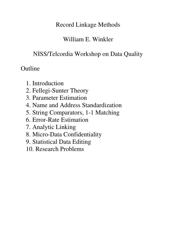
Record Linkage Methods William E. Winkler NISS/Telcordia Workshop on Data Quality Outline 1. Introduction 2. Fellegi-Sunter Theory 3. Parameter Estimation 4. Name and Address Standardization 5. String Comparators, 1-1 Matching 6. Error-Rate Estimation 7. Analytic Linking 8. Micro-Data Confidentiality 9. Statistical Data Editing 10. Research Problems

Use of Text for Classification Machine Learning Classification of Newspaper Articles into Subject Categories Classification into Disease Categories Industry and Occupation Coding Information Retrieval Library Document Search Web Search Record Linkage Identification of Duplicates Given Name, Address, Age

Model of Fellegi and Sunter ( JASA 1969) Newcombe et al. (1959), Tepping ( JASA 1968) Files A and B are matched Classify pairs from A B into Matches M and nonmatches U Each pair is a record to be classified agree/disagree – yes/no relative frequency (smith vs. zabrinsky)

If R > T µ , then designate pair as a match. If T λ < R < T µ , then designate pair as a potential match and hold for clerical review. If R < T λ , then designate pair as a nonmatch µ - bound on false match rate λ - bound on false nonmatch rate. Theorem FS (1969). Above decision rule is optimal in the sense that, for fixed bounds on the rate of false matches and nonmatches, it minimizes the clerical review region.

Conditional Independence P(agree first, agree last, agree age | M) = P(agree first | M) P(agree last |M) P(agree age| M) P(agree first, agree last, agree age | U) = P(agree first | U) P(agree last | U) P(agree age | U) No Training Data Optimal parameters vary significantly from one region to the next in the 1990 U.S. Census (Winkler ARC 1989b) Software (Winkler and Thibaudeau 1991) finds optimal yes/no parameters automatically, builds frequency tables automatically that are scaled to yes/no parameters. Entire U.S. (450 regions in 1990) matched in three weeks.

Do not need truth data set. Find optimal parameters (nearly automatically) Fellegi-Sunter (FS) – 3 variables, independence Winkler 1988 EM, independence Winkler (1989a,b, 1993) general interaction accounting for dependence, convex constraints to predispose probabilities to appropriate regions, relative frequency (Smith vs Zabrinsky) Larsen 1994, 1996 MCMC Belin and Rubin JASA 1995 EM Larsen and Rubin 2000 MCMC Some papers (e.g. Winkler rr94/05) available at http://www.census.gov/srd/www/byyear.html.

Bayesian Networks as Special Case of the Fellegi-Sunter Model of Record Linkage (FS JASA 1969, Winkler ASA 2000) Strong Statistical Basis for FS Model and Bayesian Networks Naïve Bayes – Conditional Independence Nigam, McCallum, Thrun, & Mitchell Machine Learning 2000 General Bayesian Networks (Interactions) Winkler ASA 2000

Matching Information Name Address Age John A Smith 16 Main Street 16 J H Smith 16 Main St 17 Javier Martinez 49 E Applecross Road 33 Haveir Marteenez 49 Aplecross Raod 36 Bobbie Sabin 645 Reading Aev 22 Roberta Sabin 123 Norcross Blvd Gillian Jones 645 Reading Aev 22 Jilliam Brown 123 Norcross Blvd 43 Need to see the overall lists and the context in which they are used and matched.

Name Parsing and Standardization Table Examples of Name Parsing Standardized ___ 1. DR John J Smith MD 2. Smith DRY FRM 3. Smith & Son ENTP __ Parsed PRE FIRST MID LAST POST1 POST2 BUS1 BUS2 1. DR John J Smith MD 2. Smith DRY FRM 3. Smith Son ENTP _____

Table Examples of Address Parsing Standardized_______ 1. 16 W Main ST APT 16 2. RR 2 BX 215 3. Fuller BLDG SUITE 405 4. 14588 HWY 16 W_______ Parsed (1)________ Pre2 Hsnm Stnm RR Box 1. W 16 Main 2. 2 215 3. 4. 14588 HWY 16________ Parsed (2)___________ Post1 Post2 Unit1 Unit2 Bldg 1. ST 16 2. 3. 405 Fuller 4. W_____________________

String Comparators Bigrams - Jaro JASA 1989 – insertions, deletions, transpositions Winkler 1994 – adjustments for agreements on first few characters (Pollock and Zamora CACM 1984). Table Proportional Agreement by String Comparator Values Among Matches StL Col Wash First n =1.0 0.75 0.82 0.75 � 0.6 0.93 0.94 0.93 n Last n =1.0 0.85 0.88 0.86 ✁ 0.6 0.95 0.96 0.96 n n (Smith, Smith) = 1.0 n (Dixon, Dickson) = 0.8533.

Table Comparison of String Comparators Using Last Names, First Names, and Street Names Two strings String comparator values______ Jaro Winkler Bigram SHACKLEFORD SHACKELFORD 0.970 0.982 0.700 DUNNINGHAM CUNNIGHAM 0.896 0.896 0.889 NICHLESON NICHULSON 0.926 0.956 0.625 JONES JOHNSON 0.790 0.832 0.204 MASSEY MASSIE 0.889 0.933 0.600 ABROMS ABRAMS 0.889 0.922 0.600 HARDIN MARTINEZ 0.000 0.000 0.365 ITMAN SMITH 0.000 0.000 0.250 JERALDINE GERALDINE 0.926 0.926 0.875 MARHTA MARTHA 0.944 0.961 0.400 MICHELLE MICHAEL 0.869 0.921 0.617 JULIES JULIUS 0.889 0.933 0.600 TANYA TONYA 0.867 0.880 0.500 DWAYNE DUANE 0.822 0.840 0.200 SEAN SUSAN 0.783 0.805 0.289 JON JOHN 0.917 0.933 0.408 JON JAN 0.000 0.000 0.000

✂ ✄ string comparator – model adjustment to likelihood ratios with piecewise linear functions Truth data set E.g., for each match know the string comparator values associated with comparisons of first name, last name, etc. P(1 - ((j+1)/50) n < 1 - (j/50) | M) = m j P(1 - ((j+1)/50) n < 1 - (j/50) | U) = u j for j = 1, 2, ..., 50.

1-1 Matching HouseH1 HouseH2 husband wife wife daughter daughter son son c 11 c 12 c 13 4 rows, 3 columns c 21 c 22 c 23 Take at most one in each c 31 c 32 c 33 row and column c 41 c 42 c 43 c ij is the (total agreement) weight from matching the ith person from the first file with the jth person in the second file. Stat. Can. 1987 – greedy algorithm Jaro 1989 – lsap of Burkard & Derigs 1980 Winkler 1994 – mlsap – same speed as Burkard-Derigs, storage reduced by factor of 500 (100 mB to 0.2 mB), less error

Error Rate Estimation Belin-Rubin JASA 1995 – Training data to get crude idea of shape of curves. X -Cox transform. EM to get parameters. Works well in some situations (Scheuren and Winkler 1993). 1-1 matching. No Training Data – Non-1-1 Matching Winkler 1993 – Fit interactions. Estimated error rates are accurate No Training Data – 1-1 Matching Winkler ASA 1994 EM + ad hoc Larsen ASA 1996 MCMC + ad hoc Both less accurate than BR, applicable in more situations

Blocking Soundex and NYSIIS encoding of names The methods are intended to account for very minor typographical variations. NYSIIS is used in many variants of record linkage systems. NYSIIS provides substantially more codes than Soundex. Soundex is easier to describe. Soundex consists of 4 characters. The first character agrees with the first character of the string such as surname that is being encoded. The next three characters are digits. The end of the Soundex code is ’0’ filled. Examples: Anderson, Andersen -> A536 Bergmans, Brighma -> B625 Birk, Berque, Birck -> B620 Fisher, Fischer -> F260 Lavoie, Levoy -> L100 Llwellyn -> L450 First Pass – ZIP Code + Soundex Second Pass – ZIP Code + HouseNum Third Pass – ZIP Code + Age

Estimation of False Non-Match Rates (Missed Matches) False Non-matches S 11 - captured by both blocking criteria ----------------- S 12 - captured by 1 st & not 2 nd S 11 | S 12 S 21 - captured by 2 nd & not 1 st ----------------- S 22 - captured by neither S 21 | S 22 ----------------- S 22 = S 12 S 21 / S 11 . With 3 lists, estimate S 222 . With 4 lists, estimate S 2222 . Loglinear Models (Bishop, Fienberg, & Holland 1975, Chapter 6). Example in Winkler (1989b)

Adjustment of Analyses for Matching Error where y from File A, x from File B Matching variables (name and address) uncorrelated with x and y. Methods evaluated for varying R-square values, varying amounts of overlap of Files A and B, varying amounts of matching error Scheuren and Winkler Surv. Meth. 1993 use best 2 matches Lahiri and Larsen ASA 2000 use best n matches Scheuren and Winkler Surv. Meth. 1997

Files A and B are matched. Y = Xß + .  Y i with probability p i =  Z i � Y j with probability q ij for j / =i , p i + ∑ j q ij = 1. E ( Z ) = (1/ n ) ∑ i E( Z | i ) = (1/ n ) ∑ i ( Y i p i + ∑ j Y j q ij ) = (1/ n) ∑ i Y i + (1/ n ) ∑ i [ Y i (- h i ) + Y ☎ i ) h i ] = _ + B , Y where h i = 1 - p i . Under an assumption of 1-1 matching, for each i = 1, …, n , there exists at most one j such that q ij > 0 . We let be defined by .

y where y from File A, x from File B RA RL RA EI

Linking Files for New Analyses Economics- Companies Agency A Agency B fuel ------> outputs feedstocks ------> produced Health- Individuals Receiving Agencies Social Benefits B1, B2, B3 Incomes Agency I Use of Health Agencies Services H1, H2