Randomness in Competitions Eli Ben-Naim Complex Systems Group & - PowerPoint PPT Presentation

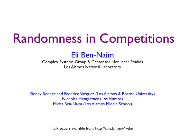
Randomness in Competitions Eli Ben-Naim Complex Systems Group & Center for Nonlinear Studies Los Alamos National Laboratory Sidney Redner and Federico Vazquez (Los Alamos & Boston University) Nicholas Hengartner (Los Alamos) Micha Ben-Naim (Los Alamos Middle School) Talk, papers available from: http://cnls.lanl.gov/~ebn

Plan 1. Modeling competitions 2. Tournaments (post season, trees) 3. Leagues (regular season, complete graphs) 4. Championships (new algorithm, regular graphs) 5. Modeling social dynamics

Motivation • Evolution: species compete, fitter wins • Society: people compete for social status • Economics: companies compete for market share • Arts, science, politics: awards, prizes, elections Competition is everywhere

Why sports? • Sports competition results are: - Accurate - Widely available - Complete Sports as a laboratory for understanding competition

Theme • Competitions are not perfectly predictable • Outcome of a single competition is stochastic • Winner of a series of competitions (league, tournament) is also subject to randomness Randomness is inherent

I. Modeling competitions

What is the most competitive sport? Soccer Baseball Hockey Basketball Football Can competitiveness be quantified? How can competitiveness be quantified?

Parity of a sports league Major League Baseball American League • Teams ranked by win-loss record 2005 Season-end Standings • Win percentage x = Number of wins Number of games • Standard deviation in win-percentage � � x 2 � − � x � 2 σ = • Cumulative distribution = Fraction of In baseball teams with winning percentage < x 0 . 400 < x < 0 . 600 F ( x ) σ = 0 . 08

Data • 300,000 Regular season games (all games ever played) • 5 Major sports leagues in United States & England sport league full name country years games soccer FA Football Association 1888-2005 43,350 baseball MLB Major League Baseball 1901-2005 163,720 hockey NHL National Hockey League 1917-2005 39,563 basketball NBA National Basketball Association 1946-2005 43,254 football NFL National Football League 1922-2004 11,770 source: http://www.shrpsports.com/ http://www.the-english-football-archive.com/

Standard deviation in winning percentage 1 data σ 0.25 0.8 theory 0.20 0.210 0.15 0.6 0.150 0.10 F(x) 0.120 0.102 0.084 0.05 0.4 0 NFL NBA MLB FA NHL NBA NFL NHL MLB 0.2 • Baseball most competitive? • Football least competitive? 0 0 0.2 0.4 0.6 0.8 1 x Distribution of winning percentage clearly distinguishes sports Fort and Quirk, 1995

“Everything should be made as simple as possible but not simpler” Freeman Dyson

“Simple Physics”

The competition model • Two, randomly selected, teams play • Outcome of game depends on team record - � q = 1 / 2 random Weaker team wins with probability q<1/2 − → q = 0 deterministic - Stronger team wins with probability p>1/2 p + q = 1 � ( i + 1 , j ) probability p ( i, j ) → i > j ( i, j + 1) probability 1 − p - When two equal teams play, winner picked randomly • Initially, all teams are equal (0 wins, 0 losses) • Teams play once per unit time � x � = 1 2

Rate equation approach • Probability distribution functions g k = fraction of teams with k wins k − 1 ∞ � � G k = g j = fraction of teams with less than k wins H k = 1 − G k +1 = g j • Evolution of the probability distribution j = k +1 j =0 dt = (1 − q )( g k − 1 G k − 1 − g k G k ) + q ( g k − 1 H k − 1 − g k H k ) + 1 dg k g 2 k − 1 − g 2 � � k 2 better team wins worse team wins equal teams play • Closed equations for the cumulative distribution dG k G 2 k − 1 − G 2 � � = q ( G k − 1 − G k ) + (1 / 2 − q ) k dt Boundary Conditions Initial Conditions G k ( t = 0) = 1 G 0 = 0 G ∞ = 1 Nonlinear Difference-Differential Equations

An exact solution • Stronger always wins (q=0) dG k = G k ( G k − G k − 1 ) dt • Transformation into a ratio P k G k = P k +1 • Nonlinear equations reduce to linear recursion dP k dt = P k − 1 • Exact solution 2! t 2 + · · · + 1 1 + t + 1 k ! t k G k = 2! t 2 + · · · + 1 + t + 1 1 ( k +1)! t k +1

Long-time asymptotics • Long-time limit 1 0.8 G k → k + 1 t • Scaling form 0.6 F(x) � k � 0.4 t=10 G k → F t=20 t t=100 0.2 • Scaling function scaling theory 0 0 1 2 0.5 1.5 F ( x ) = x x Seek similarity solutions Use winning percentage as scaling variable

Scaling analysis • Rate equation dG k G 2 k − 1 − G 2 � � = q ( G k − 1 − G k ) + (1 / 2 − q ) k dt • Treat number of wins as continuous G k +1 − G k → ∂ G ∂ k Inviscid Burgers equation ∂ G ∂ t + [ q + (1 − 2 q ) G ] ∂ G ∂ v ∂ t + v ∂ v ∂ k = 0 ∂ x = 0 • Stationary distribution of winning percentage x = k G k ( t ) → F ( x ) t • Scaling equation [( x − q ) − (1 − 2 q ) F ( x )] dF dx = 0

Scaling solution • Stationary distribution of winning percentage F ( x )  0 0 < x < q 1   x − q  q < x < 1 − q F ( x ) = 1 − 2 q   1 1 − q < x.  x • Distribution of winning percentage is uniform 1 − q q f ( x )  0 0 < x < q   1  f ( x ) = F ′ ( x ) = q < x < 1 − q 1 1 − 2 q 2 q − 1   0 1 − q < x.  x • Variance in winning percentage 1 − q q σ = 1 / 2 − q � q = 1 / 2 perfect parity √ − → q = 0 maximum disparity 3

Approach to scaling Numerical integration of the rate equations, q=1/4 1 0.5 League games Theory MLB 160 0.8 t=100 NFL 0.4 t=500 FA 40 t − 1 / 2 NHL 80 0.6 F(x) NBA 80 � 0.3 MLB NFL 16 t − 1 / 2 0.4 1 0.2 √ 4 3 0.2 0.1 0 0 200 400 600 800 1000 0 0.2 0.4 0.6 0.8 1 x t • Winning percentage distribution approaches scaling solution • Correction to scaling is very large for realistic number of games • Large variance may be due to small number of games σ ( t ) = 1 / 2 − q Large! + f ( t ) √ 3 Variance inadequate to characterize competitiveness!

The distribution of win percentage 1 0.8 0.6 F(x) 0.4 NFL NBA NHL MLB 0.2 0 0 0.2 0.4 0.6 0.8 1 x • Treat q as a fitting parameter, time=number of games • Allows to estimate q model for different leagues

The upset frequency • Upset frequency as a measure of predictability q = Number of upsets Number of games • Addresses the variability in the number of games • Measure directly from game-by-game results - Ties: count as 1/2 of an upset (small effect) - Ignore games by teams with equal records - Ignore games by teams with no record

The upset frequency 0.48 League q model q 0.46 FA 0.459 0.452 0.44 MLB 0.413 0.441 0.42 NHL 0.383 0.414 NBA 0.316 0.365 0.40 q NFL 0.309 0.364 0.38 q differentiates 0.36 FA MLB the different 0.34 NHL NBA sport leagues! 0.32 NFL 0.30 1900 1920 1940 1960 1980 2000 year Soccer, baseball most competitive Basketball, football least competitive

Evolution with time 0.48 0.28 0.26 0.46 NFL 0.24 0.44 NBA NHL 0.22 0.42 MLB 0.20 FA 0.40 q � 0.18 0.38 0.16 0.36 FA 0.14 MLB 0.34 NHL 0.12 NBA 0.32 NFL 0.10 0.30 0.08 1900 1920 1940 1960 1980 2000 1900 1920 1940 1960 1980 2000 year year • Parity, predictability mirror each other σ = 1 / 2 − q √ 3 • Football, baseball increasing competitiveness • Soccer decreasing competitiveness (past 60 years) S.J. Gould, Full House, The spread of excellence from Pluto to Darwin, 1996

I. Discussion • Model limitation: it does not incorporate - Game location: home field advantage - Game score - Upset frequency dependent on relative team strength - Unbalanced schedule • Model advantages: - Simple, involves only 1 parameter - Enables quantitative analysis

1. Conclusions • Parity characterized by variance in winning percentage - Parity measure requires standings data - Parity measure depends on season length • Predictability characterized by upset frequency - Predictability measure requires game results data - Predictability measure independent of season length • Two-team competition model allows quantitative modeling of sports competitions

2. Tournaments (post-season, trees)

Single-elimination Tournaments Binary Tree Structure

The competition model • Two teams play, loser is eliminated N → N/ 2 → N/ 4 → · · · → 1 • Teams have inherent strength (or fitness) x x 5 x 4 x 1 x 2 x 3 x strong weak • Outcome of game depends on team strength � probability 1 − q x 1 ( x 1 , x 2 ) → x 1 < x 2 probability q x 2

Recursive approach • Number of teams N = 2 k = 1 , 2 , 4 , 8 , . . . • = Cumulative probability distribution G N ( x ) function for teams with fitness less than x to win an N-team tournament • Closed equations for the cumulative distribution G 2 N ( x ) = 2 p G N ( x ) + (1 − 2 p ) [ G N ( x )] 2 Nonlinear Recursion Equation

Scaling properties 1 1. Scale of Winner 0.8 x ∗ ∼ N − ln 2 p/ ln 2 G N (x) 0.6 2. Scaling Function N=1 0.4 N=2 N=4 N=8 G N ( x ) → Ψ ( x/x ∗ ) 0.2 N=16 3. Algebraic Tail 0 0 0.2 0.4 0.6 0.8 1 x 1 − Ψ ( z ) ∼ z ln 2 p/ ln 2 q 1. Large tournaments produce strong winners 3. High probability for an upset