R Basics for Math 283 Vectors can be defined in R using the function - PowerPoint PPT Presentation
Vectors R Basics for Math 283 Vectors can be defined in R using the function c() . > x <- c(1,2,3) By Jocelyne Bruand > x Inspired by Leah Barerra's matlab tutorial [1] 1 2 3 Minor modifications by Josu Prez, Allison Wu and Glenn
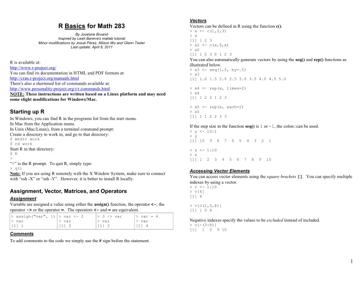
Vectors R Basics for Math 283 Vectors can be defined in R using the function c() . > x <- c(1,2,3) By Jocelyne Bruand > x Inspired by Leah Barerra's matlab tutorial [1] 1 2 3 Minor modifications by Josué Pérez, Allison Wu and Glenn Tesler > x2 <- c(x,0,x) Last update: April 8, 2011 > x2 [1] 1 2 3 0 1 2 3 You can also automatically generate vectors by using the seq() and rep() functions as R is available at: illustrated below. http://www.r-project.org/ > x3 <- seq(1,5, by=.5) You can find its documentation in HTML and PDF formats at: > x3 http://cran.r-project.org/manuals.html [1] 1.0 1.5 2.0 2.5 3.0 3.5 4.0 4.5 5.0 There's also a shortened list of commands available at: http://www.personality-project.org/r/r.commands.html > x4 <- rep(x, times=2) > x4 NOTE: These instructions are written based on a Linux platform and may need [1] 1 2 3 1 2 3 some slight modifications for Windows/Mac. > x5 <- rep(x, each=2) Starting up R > x5 [1] 1 1 2 2 3 3 In Windows, you can find R in the programs list from the start menu. In Mac from the Application menu. If the step size in the function seq() is 1 or -1 , the colon : can be used. In Unix (Mac/Linux), from a terminal command prompt: > y <- 10:1 Create a directory to work in, and go to that directory: > y $ mkdir work [1] 10 9 8 7 6 5 4 3 2 1 $ cd work Start R in that directory: > z <- 1:10 $ R > z > [1] 1 2 3 4 5 6 7 8 9 10 “>” is the R prompt. To quit R, simply type: > q() Accessing Vector Elements Note: If you are using R remotely with the X Window System, make sure to connect You can access vector elements using the square brackets [] . You can specify multiple with “ssh -X” or “ssh -Y”. However, it is better to install R locally. indexes by using a vector. > v <- 1:10 Assignment, Vector, Matrices, and Operators > v[6] [1] 6 Assignment Variable are assigned a value using either the assign() function, the operator <- , the > v[c(1,5,8)] operator -> or the operator = . The operators <- and = are equivalent. [1] 1 5 8 > assign("var", 1) > var <- 2 > 3 -> var > var = 4 Negative indexes specify the values to be excluded instead of included. > var > var > var > var > v[-(3:8)] [1] 1 [1] 2 [1] 3 [1] 4 [1] 1 2 9 10 Comments To add comments to the code we simply use the # sign before the statement. 1
Operators Arithmetic operators in R Arrays and Matrices * / + - ^ You can create matrices by using the array() function, which takes the form array( data_vector , dim_vector ) . If there are less values in the data vector than the are element-by-element operators , and follow the expected order of operations. dimension of the array calls for, then the values are recycled. > 12/3+4^5-4^5 [1] 4 > array(1:4, c(2,2)) [,1] [,2] [1,] 1 3 In order to do matrix operations which follow the rules of linear algebra, you must use [2,] 2 4 the following operators ( %*% is the dot product (inner product) and %o% is the outer > array(1:4, c(2,3)) [,1] [,2] [,3] matrix multiplication): [1,] 1 3 1 %*% %o% [2,] 2 4 2 Here's what a few operators would return: > array(0, c(2,2)) [,1] [,2] > x <- c(1,2,3) [1,] 0 0 > y <- c(4,5,6) [2,] 0 0 > x+y [1] 5 7 9 Accessing Array Elements Array elements can be accessed in the same way as vectors. > x-y [1] -3 -3 -3 > A <- array(1:4, c(2,2)) > x*y [1] 4 10 18 [,1] [,2] [1,] 1 3 > x/y [1] 0.25 0.40 0.50 [2,] 2 4 > x^y [1] 1 32 729 A[i] accesses the i-th element in matrix A (going by columns). > x%*%y [,1] > A[3] [1] 3 [1,] 32 A[i,] accesses the i-th row in matrix A . > x%o%y [,1] [,2] [,3] > A[1,] [1] 1 3 [1,] 4 5 6 A[,j] accesses the j-th column in matrix A . [2,] 8 10 12 > A[,1] [1] 1 2 [3,] 12 15 18 Note that a vector does not have a “direction”, i.e. the function c() does not create row A[i,j] accesses the element in the i-th row, j-th column in A . vectors or column vectors, just vectors. > A[1,2] [1] 3 More Basic Operators/Functions exp log log10 log2 sqrt Also, you can create matrices by using matrix ( data_vector, number_rows, number of cols) . For example: > j <- matrix(1:4, 2, 2) Workspace and File Management > j The following functions manage your file system and the variables in your R workspace. [,1] [,2] browse.workspace() creates a window with information about all variables in the [1,] 1 3 workspace [2,] 2 4 ls() list the variables in the workspace rm(x) remove x from the workspace Accessing the elements remains the same no matter the function used to create the matrix. rm(list=ls()) remove all the variables from the workspace dir() list the directory/files of the current directory. Some Basic Functions on Vectors and Arrays setwd(my_dir) change current working directory to my_dir Type ‘help( function_name ) ’ for details on usage. unlink(filename) deletes the file filename . dim t max min mean var sd sort sum prod diff 2
Reading/Writing Data from/to a File You can use the data frame like a matrix, but if you want to convert it back to a matrix, Data frames you can do that in the following way: R encourages the use of data frames which are matrices in which each column has a title and can be of a different type. > array(unlist(A, use.names=FALSE), dim(A)) > df <- data.frame(name=c("Joe", "Tom"), age=c(21,22)) > df Or the command: name age 1 Joe 21 > matrix(unlist(A, use.names=FALSE), dim(A)) 2 Tom 22 Writing data to file With either command the output would be: The function write.table() allows to write data to a file. However, all will be converted to a data frame first. [,1] [,2] > write.table(df, file="example.txt") [1,] 1 3 example.txt: [2,] 2 4 "name" "age" "1" "Joe" 21 Control Flow "2" "Tom" 22 Conditional Control – if, else, ifelse Conditional control is achieved using the if/else statements. Notice how R added row labels for you. This can be a problem when trying to write a > if ( expr_1 ) expr_2 else expr_3 matrix to a file: This first evaluates expr_1 . If it is true, then expr_2 is executed, otherwise, expr_3 is > write.table(array(1:4, c(2,2)), file="example.txt") example.txt: executed. There is a vectorized version of the if/else construct, the ifelse() function. This has the "V1" "V2" form ifelse(condition, a, b) and returns a vector of the length of its longest argument, "1" 1 3 with elements a[i] if condition[i] is true, otherwise b[i]. "2" 2 4 > x <- 0 > if (x == 0) x = 1 else x = 2 Luckily, if you do not want to deal with data frames, there is a way around it: > x write.table(array(1:4, c(2,2)), file="example.txt", [1] 1 row.names=FALSE, col.names=FALSE) example.txt: > if (x == 0) x = 1 else x = 2 > x 1 3 [1] 2 2 4 Reading data from file > ifelse(c(TRUE, FALSE), c(1,1), c(2,2)) Data files can be read using the table.read() function. [1] 1 2 Let us take the last file we wrote. example.txt: Repetitive Execution – for, while, break 1 3 Statements can be repeated a specific number of times using for loops. 2 4 > for (name in expr_1 ) expr_2 This causes name to iterate through a vector expr_1 and execute expr_2 for each value Then, we can read its content in the following manner. of name . > A <- read.table("example.txt") For example, we could add the numbers from 1 to 10: > A > x <- 0 V1 V2 > for(i in 1:10) x = x+i 1 1 3 > x 2 2 4 [1] 55 3
Recommend
More recommend
Explore More Topics
Stay informed with curated content and fresh updates.
