Quantum pattern matching fast on average Ashley Montanaro - PowerPoint PPT Presentation

Quantum pattern matching fast on average Ashley Montanaro Department of Computer Science, University of Bristol, UK 12 January 2015

Pattern matching In the traditional pattern matching problem, we seek to find a pattern P : [ m ] → Σ within a text T : [ n ] → Σ . Q U A N T = T U M P = A N T

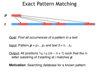
Pattern matching In the traditional pattern matching problem, we seek to find a pattern P : [ m ] → Σ within a text T : [ n ] → Σ . Q U A N T = T U M P = A N T

Pattern matching In the traditional pattern matching problem, we seek to find a pattern P : [ m ] → Σ within a text T : [ n ] → Σ . Q U A N T = T U M P = A N T We can generalise this to higher dimensions d , where P : [ m ] d → Σ and T : [ n ] d → Σ : T = P =

Pattern matching Focusing on the 1-dimensional problem for now: Classically, it is known that this problem can be solved in worst-case time O ( n + m ) [Knuth, Morris and Pratt ’77] .

Pattern matching Focusing on the 1-dimensional problem for now: Classically, it is known that this problem can be solved in worst-case time O ( n + m ) [Knuth, Morris and Pratt ’77] . There is a quantum algorithm which solves this problem (with bounded failure probability) in time O ( √ n + √ m ) [Ramesh and Vinay ’03] . �

Pattern matching Focusing on the 1-dimensional problem for now: Classically, it is known that this problem can be solved in worst-case time O ( n + m ) [Knuth, Morris and Pratt ’77] . There is a quantum algorithm which solves this problem (with bounded failure probability) in time O ( √ n + √ m ) [Ramesh and Vinay ’03] . � Both these bounds are optimal in the worst case. But. . . what about the average case?

Pattern matching Focusing on the 1-dimensional problem for now: Classically, it is known that this problem can be solved in worst-case time O ( n + m ) [Knuth, Morris and Pratt ’77] . There is a quantum algorithm which solves this problem (with bounded failure probability) in time O ( √ n + √ m ) [Ramesh and Vinay ’03] . � Both these bounds are optimal in the worst case. But. . . what about the average case? Consider a simple model where each character of T is picked uniformly at random from Σ , and either: P is chosen to be an arbitrary substring of T ; or P is uniformly random. Could this be easier?

Pattern matching Classically, one can solve the average-case problem in time O ( n / m + √ n ) , and this is optimal. �

Pattern matching Classically, one can solve the average-case problem in time O ( n / m + √ n ) , and this is optimal. � But in the quantum setting, we have the following result: Theorem (modulo minor technicalities) Let T : [ n ] → Σ , P : [ m ] → Σ be picked as on the previous slide. Then there is a quantum algorithm which runs in time n / m 2 O ( √ � � log m ) ) O ( and determines whether P matches T .

Pattern matching Classically, one can solve the average-case problem in time O ( n / m + √ n ) , and this is optimal. � But in the quantum setting, we have the following result: Theorem (modulo minor technicalities) Let T : [ n ] → Σ , P : [ m ] → Σ be picked as on the previous slide. Then there is a quantum algorithm which runs in time n / m 2 O ( √ � � log m ) ) O ( and determines whether P matches T . If P does match T , the algorithm also outputs the position at which the match occurs.

Pattern matching Classically, one can solve the average-case problem in time O ( n / m + √ n ) , and this is optimal. � But in the quantum setting, we have the following result: Theorem (modulo minor technicalities) Let T : [ n ] → Σ , P : [ m ] → Σ be picked as on the previous slide. Then there is a quantum algorithm which runs in time n / m 2 O ( √ � � log m ) ) O ( and determines whether P matches T . If P does match T , the algorithm also outputs the position at which the match occurs. The algorithm fails with probability O ( 1 / n ) , taken over both the choice of T and P , and its internal randomness.

Pattern matching Classically, one can solve the average-case problem in time O ( n / m + √ n ) , and this is optimal. � But in the quantum setting, we have the following result: Theorem (modulo minor technicalities) Let T : [ n ] → Σ , P : [ m ] → Σ be picked as on the previous slide. Then there is a quantum algorithm which runs in time n / m 2 O ( √ � � log m ) ) O ( and determines whether P matches T . If P does match T , the algorithm also outputs the position at which the match occurs. The algorithm fails with probability O ( 1 / n ) , taken over both the choice of T and P , and its internal randomness. This is a super-polynomial speedup for large m .

Pattern matching ( d -dimensional) Classically, one can solve the average-case problem in time O (( n / m ) d + n d / 2 ) , and this is optimal. � But in the quantum setting, we have the following result: Theorem (modulo minor technicalities) Let T : [ n ] d → Σ , P : [ m ] d → Σ be picked as on the previous slide. Then there is a quantum algorithm which runs in time O (( n / m ) d / 2 2 O ( d 3 / 2 √ � log m ) ) and determines whether P matches T . If P does match T , the algorithm also outputs the position at which the match occurs. The algorithm fails with probability O ( 1 / n d ) , taken over both the choice of T and P , and its internal randomness. This is a super-polynomial speedup for large m .

The dihedral hidden subgroup problem The main quantum ingredient in the algorithm is an algorithm for the dihedral hidden subgroup problem (aka finding hidden shifts over Z N ): Given two injective functions f , g : Z N → X such that g ( x ) = f ( x + s ) for some s ∈ Z N , determine s .

The dihedral hidden subgroup problem The main quantum ingredient in the algorithm is an algorithm for the dihedral hidden subgroup problem (aka finding hidden shifts over Z N ): Given two injective functions f , g : Z N → X such that g ( x ) = f ( x + s ) for some s ∈ Z N , determine s . The best known quantum algorithm for the dihedral HSP uses 2 O ( √ log N ) = o ( N ǫ ) queries [Kuperberg ’05] . √ Classically, there is a lower bound of Ω ( N ) queries.

From the dihedral HSP to pattern matching Can we treat f and g as text and pattern, and use the dihedral HSP to solve the general pattern matching problem?

From the dihedral HSP to pattern matching Can we treat f and g as text and pattern, and use the dihedral HSP to solve the general pattern matching problem? The dihedral HSP algorithm requires the pattern and text to be. . . injective the same length 1-dimensional Also, a different notion of shifts is used (modulo N ).

From the dihedral HSP to pattern matching Can we treat f and g as text and pattern, and use the dihedral HSP to solve the general pattern matching problem? The dihedral HSP algorithm requires the pattern and text to be. . . injective the same length 1-dimensional Also, a different notion of shifts is used (modulo N ). Can we relax these assumptions?

From the dihedral HSP to pattern matching First, we make the pattern and text injective by concatenating characters (an idea used previously in some different contexts [Knuth ’77, Gharibi ’13] ): Q QU UA AN NT TU UM U A N T U M A N T AN NT

From the dihedral HSP to pattern matching First, we make the pattern and text injective by concatenating characters (an idea used previously in some different contexts [Knuth ’77, Gharibi ’13] ): Q QU UA AN NT TU UM U A N T U M A N T AN NT Concatenation preserves the property of the pattern matching the text.

From the dihedral HSP to pattern matching First, we make the pattern and text injective by concatenating characters (an idea used previously in some different contexts [Knuth ’77, Gharibi ’13] ): Q QU UA AN NT TU UM U A N T U M A N T AN NT Concatenation preserves the property of the pattern matching the text. If we produce a new alphabet whose symbols are strings of length k , a query to the new string can be simulated by k queries to the original string.

From the dihedral HSP to pattern matching First, we make the pattern and text injective by concatenating characters (an idea used previously in some different contexts [Knuth ’77, Gharibi ’13] ): Q QU UA AN NT TU UM U A N T U M A N T AN NT Concatenation preserves the property of the pattern matching the text. If we produce a new alphabet whose symbols are strings of length k , a query to the new string can be simulated by k queries to the original string. For most random strings, it suffices to take k = O ( log n ) .

From the dihedral HSP to pattern matching Second, we apply the dihedral HSP algorithm to the (now injective) pattern and text, at a randomly chosen offset.

From the dihedral HSP to pattern matching Second, we apply the dihedral HSP algorithm to the (now injective) pattern and text, at a randomly chosen offset.

From the dihedral HSP to pattern matching Second, we apply the dihedral HSP algorithm to the (now injective) pattern and text, at a randomly chosen offset. Claim If the pattern is contained in the text, and our guess for the start of the pattern is correct to within distance m 2 − O ( √ log m ) , the dihedral HSP algorithm outputs the correct shift with high probability.

Completing the argument ( d = 1 ) The probability of our guess being in this “good” range is p = Ω ( m 2 − O ( √ log m ) / n ) .