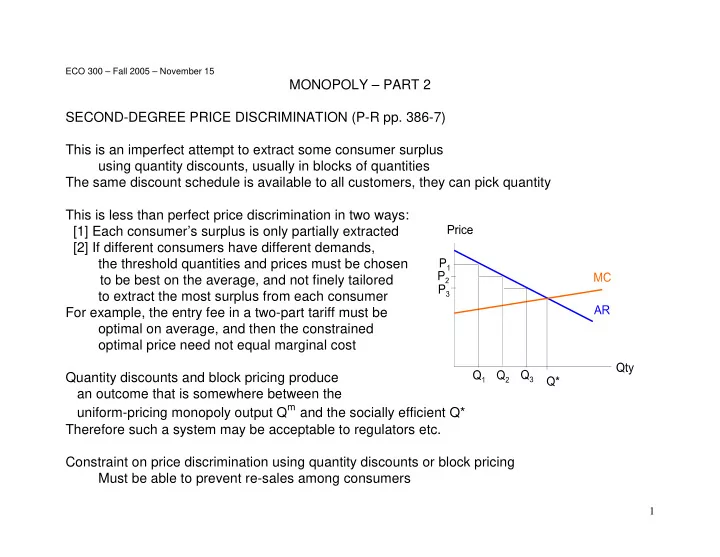

ECO 300 – Fall 2005 – November 15 MONOPOLY – PART 2 SECOND-DEGREE PRICE DISCRIMINATION (P-R pp. 386-7) This is an imperfect attempt to extract some consumer surplus using quantity discounts, usually in blocks of quantities The same discount schedule is available to all customers, they can pick quantity This is less than perfect price discrimination in two ways: [1] Each consumer’s surplus is only partially extracted [2] If different consumers have different demands, the threshold quantities and prices must be chosen to be best on the average, and not finely tailored to extract the most surplus from each consumer For example, the entry fee in a two-part tariff must be optimal on average, and then the constrained optimal price need not equal marginal cost Quantity discounts and block pricing produce an outcome that is somewhere between the uniform-pricing monopoly output Q m and the socially efficient Q* Therefore such a system may be acceptable to regulators etc. Constraint on price discrimination using quantity discounts or block pricing Must be able to prevent re-sales among consumers 1
THIRD-DEGREE PRICE DISCRIMINATION – “GROUPING” AT SELLER’S DISCRETION (P-R pp. 388-90) Identify different groups with different demands (importantly, different elasticities) and charge separate different prices to each Two groups, inverse demand functions P 1 = D 1 (Q 1 ) and P 2 = D 2 (Q 2 ) . Write Q = Q 1 + Q 2 Monopolist wants to maximize profit B = P 1 Q 1 + P 2 Q 2 – C(Q) Condition for optimal Q 1 (similar condition for Q 2 ) ∂ ⎛ ⎞ Q dP dC Q 1 + − = = − ⎟ = ⎜ 1 P 0 , or MR MC , or P 1 MC ∂ ⎝ ⎠ 1 1 1 1 dQ dQ Q e 1 1 1 e e = = 1 2 P MC , P MC Then − − 1 2 e 1 e 1 1 2 Numerical example: If e 1 = 5 and e 2 = 10, then P 1 = 1.25 MC and P 2 = 1.11 MC Group with less elastic demand pays higher price Examples – [1] Students’ demand for textbooks is very price inelastic When campus stores hold sales, they usually exclude textbooks [2] New customers are more price-sensitive than returning ones So introductory discounts are more common than renewal discounts 2
THIRD-DEGREE PRICE DISCRIMINATION – “VERSIONING” & BUYERS’ SELF-SELECTION Here the firm does not know the group membership of any individual customer and so cannot present him with just the price intended for that group (or is not legally allowed to do so) Instead, the firm designs two (or more) different purchase contracts in such a way that each group’s members will self-select the one that was intended for them Examples – restricted vs. unrestricted air fares, hardback vs. paperback books, ... (Quantity discount or block pricing schedules can also have this purpose) Numerical example – Pie-In-The-Sky (PITS) airline’s route between Podunk and Wobegon 100 potential customers each day; 70 tourist, 30 business Each buys at most one ticket. Max willingness to pay for it is called “reservation price” Reservation price PITS’s potential profit Type of PITS’s ticket cost Tourist Business Tourist Business Restricted 100 140 225 40 125 Unrestricted 150 175 300 25 150 Perfect price discrimination: Sell R to each T at 140, sell U to each B at 300 Profit = (140–100) * 70 + (300–150) * 30 = 40 * 70 + 150 * 30 = 2800 + 4500 = 7300 Various strategies compatible with PITS’s available information : [1] R only - Either price at 140, profit 40 * 100 = 4000, or price at 225, profit = 125 * 30 = 3750 [2] U only - Either price at 175, profit 25 * 100 = 2500, or price at 300, profit = 150 * 30 = 4500 3
[3] Both, priced R at X, U at Y, to be determined Each type of customer will buy the ticket that yields larger consumer surplus Assume that each type B or T, when surpluses equal, will choose U Want T to choose R : 140 – X > 175 – Y, or Y – X > 35 Want B to choose U : 225 – X < 300 – Y, or Y – X < 75 These give each type of consumer the right incentive to choose the type of ticket the airline wants him to choose – Therefore they are called the “incentive-compatibility” or “self-selection” constraints Figure shows them in green The airline must also set X < 140, else T doesn’t buy R, Y < 300, else B doesn’t buy U These are called “individual rationality” or “participation” constraints Figure shows them in blue So overall feasible region for choice of X, Y is the shaded area 4
PITS’ profit is 70 ( X - 100 ) + 30 ( Y - 150 ) = 70 X + 30 Y - 11,500 Therefore PITS’ iso-profit lines have equations 70 X + 30 Y = constant; they are shown in red PITS’ optimal choice is X = 140, Y = 215, shown by bullet Resulting profit = (140–100) * 70 + (215–150) * 30 = 2800 + 1950 = 4750 Better than that of any of the single type of service strategies in [1] and [2] But less than the 7300 PITS could make if it could identify individuals’ types and use this information to implement perfect price discrimination So the “versioning” strategy lets PITS increase its profit above single-type strategies by extracting some but not all consumer surplus Each T-type still gets almost no surplus. But each B-type gets 300 – 215 = 85; PITS can’t charge them more than 215; they would buy R tickets, even worse for PITS. This is PITS’s cost of its information disadvantage (not knowing individuals’ group identity) In the language of the economics of asymmetric information (more later in course) this is an example of “screening by self-selection” P-R’s analysis of bundling in restaurant menus (pp. 404-414) is another example 5
Recommend
More recommend