Propagation of Interval and What We Do in This . . . Probabilistic - PowerPoint PPT Presentation
Need for Data . . . Need to Take . . . Measurement . . . Propagation of . . . Propagation of Interval and What We Do in This . . . Probabilistic Uncertainty in Chapter 2: Towards . . . Chapter 3: Towards . . . Cyberinfrastructure-Related
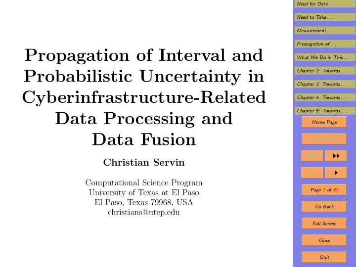
Need for Data . . . Need to Take . . . Measurement . . . Propagation of . . . Propagation of Interval and What We Do in This . . . Probabilistic Uncertainty in Chapter 2: Towards . . . Chapter 3: Towards . . . Cyberinfrastructure-Related Chapter 4: Towards . . . Chapter 5: Towards . . . Data Processing and Home Page Data Fusion Title Page ◭◭ ◮◮ Christian Servin ◭ ◮ Computational Science Program Page 1 of 65 University of Texas at El Paso El Paso, Texas 79968, USA Go Back christians@utep.edu Full Screen Close Quit
Need for Data . . . Need to Take . . . 1. Need for Data Processing and Data Fusion Measurement . . . • For many quantities y , it is not easy (or even impossi- Propagation of . . . ble) to measure them directly. What We Do in This . . . Chapter 2: Towards . . . • Instead, we measure related quantities x 1 , . . . , x n , and Chapter 3: Towards . . . use the known relation y = f ( x 1 , . . . , x n ) to estimate y . Chapter 4: Towards . . . • Such data processing is especially important for Chapter 5: Towards . . . cyberinfrastructure-related heterogenous data. Home Page • Example of heterogenous data – geophysics: Title Page – first-arrival passive (from actual earthquakes) and ◭◭ ◮◮ active seismic data (from seismic experiments); ◭ ◮ – gravity data; Page 2 of 65 – surface waves, etc. Go Back • Before we start processing data, we need to first fuse Full Screen data points corresponding to the same quantity. Close Quit
Need for Data . . . Need to Take . . . 2. Need to Take Uncertainty into Consideration Measurement . . . • The result � x of a measurement is usually somewhat Propagation of . . . different from the actual (unknown) value x . What We Do in This . . . Chapter 2: Towards . . . • Usually, the manufacturer of the measuring instrument Chapter 3: Towards . . . (MI) gives us a bound ∆ on the measurement error: Chapter 4: Towards . . . def | ∆ x | ≤ ∆ , where ∆ x x − x = � Chapter 5: Towards . . . Home Page • Once we know the measurement result � x , we can con- x − ∆ , � clude that the actual value x is in [ � x + ∆]. Title Page ◭◭ ◮◮ • In some situations, we also know the probabilities of different values ∆ x ∈ [ − ∆ , ∆]. ◭ ◮ • In this case, we can use statistical techniques. Page 3 of 65 • However, often, we do not know these probabilities; we Go Back def only know that x is in the interval x = [ � x − ∆ , � x + ∆]. Full Screen • In this case, we need to process this interval data. Close Quit
Need for Data . . . Need to Take . . . 3. Measurement Uncertainty: Traditional Approach Measurement . . . def • Usually, a meas. error ∆ x = � x − x is subdivided into Propagation of . . . random and systematic components ∆ x = ∆ x s + ∆ x r : What We Do in This . . . Chapter 2: Towards . . . – the systematic error component ∆ x s is usually de- Chapter 3: Towards . . . fined as the expected value ∆ x s = E [∆ x ], while Chapter 4: Towards . . . – the random error component is usually defined as Chapter 5: Towards . . . def the difference ∆ x r = ∆ x − ∆ x s . Home Page • The random errors ∆ x r corresponding to different mea- Title Page surements are usually assumed to be independent. ◭◭ ◮◮ • For ∆ x s , we only know the upper bound ∆ s s.t. ◭ ◮ | ∆ x s | ≤ ∆ s , i.e., that ∆ x s is in the interval [ − ∆ s , ∆ s ]. Page 4 of 65 • Because of this fact, interval computations are used for processing the systematic errors. Go Back Full Screen • ∆ x r is usually characterized by the corr. probability distribution (usually Gaussian, with known σ ). Close Quit
Need for Data . . . Need to Take . . . 4. Expert Estimates and Fuzzy Data Measurement . . . • There is no guarantee of expert’s accuracy. Propagation of . . . What We Do in This . . . • We can only provide bounds which are valid with some Chapter 2: Towards . . . degree of certainty. Chapter 3: Towards . . . • This degree of certainty is usually described by a num- Chapter 4: Towards . . . ber from the interval [0 , 1]. Chapter 5: Towards . . . • So, for each β ∈ [0 , 1], we have an interval x ( α ) con- Home Page taining the actual value x with certainty α = 1 − β . Title Page • The larger certainty we want, the broader should the ◭◭ ◮◮ corresponding interval be. ◭ ◮ • So, we get a nested family of intervals corresponding Page 5 of 65 to different values α . Go Back • Alternative: for each x , describe the largest α for which Full Screen x is in x ( α ); this α largest is a membership function µ ( x ). Close Quit
Need for Data . . . Need to Take . . . 5. How to Propagate Uncertainty in Data Pro- Measurement . . . cessing Propagation of . . . • We know that y = f ( x 1 , . . . , x n ). What We Do in This . . . Chapter 2: Towards . . . • We estimate y based on the approximate values � x i as Chapter 3: Towards . . . y = f ( � � x 1 , . . . , � x n ). Chapter 4: Towards . . . • Since � x i � = x i , we get � y � = y ; it is desirable to estimate Chapter 5: Towards . . . def the approximation error ∆ y = � y − y . Home Page • Usually, measurements are reasonably accurate, i.e., Title Page def measurement errors ∆ x i = � x i − x i are small. ◭◭ ◮◮ • Thus, we can keep only linear terms in Taylor expan- ◭ ◮ � n C i · ∆ x i , where C i = ∂f sion: ∆ y = . ∂x i Page 6 of 65 i =1 � n Go Back • For systematic error, we get a bound | C i | · ∆ si . i =1 Full Screen � n • For random error, we get σ 2 = C 2 i · σ 2 i . Close i =1 Quit
Need for Data . . . Need to Take . . . 6. How to Propagate Uncertainty in Data Fusion: Measurement . . . Case of Probabilistic Uncertainty Propagation of . . . x ( n ) of x (1) , . . . , � • Reminder: we have several estimates � What We Do in This . . . the same quantity x . Chapter 2: Towards . . . Chapter 3: Towards . . . • Data fusion: we combine these estimates into a single Chapter 4: Towards . . . estimate � x . Chapter 5: Towards . . . • Case: each estimation error ∆ x ( i ) def x ( i ) − x is normally = � Home Page distributed with 0 mean and known st. dev. σ ( i ) . Title Page • How to combine: use Least Squares, i.e., find � x that x ( i ) − � ◭◭ ◮◮ x ) 2 � n ( � minimizes 2 · ( σ ( i ) ) 2 ; ◭ ◮ i =1 � n Page 7 of 65 x ( i ) · ( σ ( i ) ) − 2 � Go Back i =1 • Solution: � x = . � n ( σ ( i ) ) − 2 Full Screen i =1 Close Quit
Need for Data . . . Need to Take . . . 7. Data Fusion: Case of Interval Uncertainty Measurement . . . • In some practical situations, the value x is known with Propagation of . . . interval uncertainty. What We Do in This . . . Chapter 2: Towards . . . • This happens, e.g., when we only know the upper bound ∆ ( i ) on each estimation error ∆ x ( i ) : | ∆ x ( i ) | ≤ ∆ i . Chapter 3: Towards . . . Chapter 4: Towards . . . x ( i ) | ≤ ∆ ( i ) , i.e., • In this case, we can conclude that | x − � Chapter 5: Towards . . . x ( i ) − ∆ ( i ) , � x ( i ) + ∆ ( i ) ]. that x ∈ x ( i ) def = [ � Home Page x ( i ) , we know that the actual • Based on each estimate � Title Page value x belongs to the interval x ( i ) . ◭◭ ◮◮ • Thus, we know that the (unknown) actual value x be- ◭ ◮ longs to the intersection of these intervals: Page 8 of 65 n � x ( i ) = [max( � x ( i ) − ∆ ( i ) ) , min( � x ( i ) + ∆ ( i ) )] . def Go Back x = i =1 Full Screen Close Quit
Need for Data . . . Need to Take . . . 8. Propagation of Uncertainty: Challenges Measurement . . . • In the ideal world: Propagation of . . . What We Do in This . . . – we should have an accurate description of data un- Chapter 2: Towards . . . certainty; Chapter 3: Towards . . . – based on this description, we should use well-justified Chapter 4: Towards . . . and efficient algorithms to propagate uncertainty. Chapter 5: Towards . . . • In practice , we are often not yet in this ideal situation: Home Page – the description of uncertainty is often only approx- Title Page imate , ◭◭ ◮◮ – the algorithms for uncertainty propagation are of- ◭ ◮ ten heuristics , i.e., not well-justified, and Page 9 of 65 – the algorithms for uncertainty propagation are of- Go Back ten not very computationally efficient . Full Screen Close Quit
Need for Data . . . Need to Take . . . 9. What We Do in This Thesis Measurement . . . • In Chapter 2, we show that the traditional idea of ran- Propagation of . . . dom and systematic components is an approximation : What We Do in This . . . Chapter 2: Towards . . . – we also need periodic components; Chapter 3: Towards . . . – this is important in environmental studies. Chapter 4: Towards . . . • In Chapter 3, on the example of a fuzzy heuristic , we Chapter 5: Towards . . . show how a heuristic can be formally justified . Home Page • In Ch. 4, we show how to process more efficiently ; e.g.: Title Page ◭◭ ◮◮ – first, we process data type-by-type; – then, we fuse the resulting models. ◭ ◮ Page 10 of 65 • All these results assume that we have a good descrip- tion of the uncertainty of the original data. Go Back • In practice, we often need to extract this information Full Screen from the data; these are our future plans (Ch. 5). Close Quit
Recommend
More recommend
Explore More Topics
Stay informed with curated content and fresh updates.
