Production theory: accounting for firm heterogeneity and technical - - PowerPoint PPT Presentation

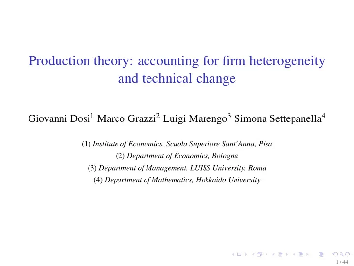
Production theory: accounting for firm heterogeneity and technical change

Giovanni Dosi1 Marco Grazzi2 Luigi Marengo3 Simona Settepanella4

(1) Institute of Economics, Scuola Superiore Sant’Anna, Pisa (2) Department of Economics, Bologna (3) Department of Management, LUISS University, Roma (4) Department of Mathematics, Hokkaido University

1 / 44

Rudimentary standard production theory

production vector y = (y1, y2, . . . , yL) ∈ RL production set (feasible techniques) Y ∈ RL a bunch of underlying heroic assumptions:

◮ closeness of Y ◮ divisibility ◮ convexity ◮ non-incresing returns to scale

strong behavioral assupmtions on the choice of techniques

◮ max p · y ◮ s.t. y ∈ Y 2 / 44

Cobb-Douglas production function

y = xα

1 xβ 2 with α + β = 1

handy link with income distribution:

∂y ∂xi = pi

p1x1 + p2x2 = y

3 / 44

Some consequences

if prices pi are common to all firms they will choose techniques with equal relative productivities thus implications for:

◮ elasticities of substitutions ◮ duality ◮ dynamics: Y(t) = A(t)f(K(t), L(t)) 4 / 44

What about the evidence?

the assumptions are unreasonable (e.g. returns to scale and related convexity) an extreme case: information the model implies that firms access the same set Y and choose the same techniques: on the contrary we observe strong heterogeneity

5 / 44

Stylized facts on heterogeneity

Robust evidence across many industries and countries (USA, Canada, UK, France, Italy, Netherlands, etc) consistently finds: wide asymmetries in productivity across firms equally wide heterogeneity in relative input intensities highly skewed distribution of efficiency, innovativeness and profitability indicators; different export status within the same industry high intertemporal persistence in the above properties high persistence of heterogeneity also when increasing the level of disaggregation

6 / 44

Disaggregation does not solve the problem

“We [...] thought that one could reduce heterogeneity by going down from general mixtures as “total manufacturing” to something more coherent, such as “petroleum refining” or “the manufacture of cement.” But something like Mandelbrot’s fractal phenomenon seems to be at work here also: the

• bserved variability-heterogeneity does not really decline as we cut our data

finer and finer. There is a sense in which different bakeries are just as much different from each others as the steel industry is from the machinery industry.” (Griliches and Mairesse, Production function: the search for identification, 1999)

7 / 44

• Heterog. performances Meat Products (1999)

0.2 0.4 0.6 0.8 1 1.2 2.5 3 3.5 4 4.5 5 5.5 Year 1999 (log) Labor Productivity Pr 151 1511 1513

exp(3) ≈ 20 th. euro; exp(4.5) ≈ 90 th. euro

8 / 44

• Heterog. in performances is persistent (year 2006)

0.2 0.4 0.6 0.8 1 1.2 2.5 3 3.5 4 4.5 5 5.5 Year 2006 (log) Labor Productivity Pr 151 1511 1513

exp(3) ≈ 20 th. euro; exp(4.5) ≈ 90 th. euro

9 / 44

• Heterog. in adopted techniques

3.5 4 4.5 5 5.5 6 6.5 3 4 5 6 7 8 9 5 6 7 8 9 10 11 12 ISIC 151 log VA log L log K

10 / 44

Remarks

heterogeneity of productivities under similar relative prices even more heterogeneity across countries not reducible a scalar difference among production functions

11 / 44

This is challenging....

This evidence poses serious challenges to theoretical and/or empirical analyses which rely upon some notion of industries as aggregates of similar/homogeneous production units: models based on industry production function empirical exercises based on some notion of efficiency frontier but also sectoral input-output coefficient à la Leontief are meaningless if computed as averages over such very dispersed and skewed distributions indicators of technical change based on variations of such aggregates (isoquants or input-output coefficients) may be seriously misleading

12 / 44

Toward an alternative theory of production

1

theories of arrival and adoption of techniques (evolutionary theories of innovation)

2

synthetic representations of the actual distribution of techniques, their properties, and their dynamics

13 / 44

Our attempt

Can we give a representation of the production technology(ies) of an industry fully taking into account heterogeneity? ... and without imposing any hypothesis on functional forms or input substitutions which do not have empirical ground? Can we produce empirical measures of the technological characteristics

• f an industry which explicitly take into account heterogeneity?
• ur attempt goes back and develops upon W. Hildenbrand “Short-run

production functions based on microdata” Econometrica, 1981

14 / 44

Hildenbrand’s analysis

Represent firms in one sector as empirical input-output vectors of production at full capacity with some weak additional assumptions (divisibility) derives the empirical production possibility set for the industry (geometrically, a zonotope) and shows the following main properties of the derived efficiency frontier:

◮ returns to scale are never constant ◮ the elasticities of substitution are not constant 15 / 44

Our contribution

Building upon Hildenbrand (1981) we derive: indicators of industry heterogeneity rigorous measures of technical change at the industry level which do not assume any averaging out of heterogeneity

◮ rate and direction of technical change

Industry dynamics: how firm entry and exit affects heterogeneity and tech change We provide an application on Italian industrial census data Compare with existing measure of productivity

16 / 44

Production activities and Zonotopes

The ex post technology of a production unit is a vector a = (α1, . . . , αl, αl+1) ∈ Rl+1

+ ,

i.e. a production activity a that produces, during the current period, αl+1 units of output by means of (α1, . . . , αl) units of input.

◮ Holds also also for the multi-output case

The size of the firm is the length of vector a, i.e. a multi-dimensional extension of the usual measure of firm size. The short run production possibilities of an industry with N units at a given time is a finite family of vectors {an}1≤n≤N of production activities Hildenbrand defines the short run total production set associated to them as the Zonotope Y = {y ∈ Rl+1

+

| y =

N

• n=1

φnan, 0 ≤ φn ≤ 1}.

17 / 44

Production activities in a 3-dimensional space

2 4 6 8 10 0 2 4 6 8 10 2 4 6 8 10 E m p l

• y

e e s Tangible assets VA

18 / 44

The Zonotope

19 / 44

Zonotope generated by 300 random vectors

20 / 44

Volume of Zonotopes and Gini index

The volume of the zonotope Y in Rl+1 is given by: Vol(Y) =

• 1≤i1<...<il+1≤N

| ∆i1,...,il+1 | where | ∆i1,...,il+1 | is the module of the determinant ∆i1,...,il+1. Interested in getting an absolute measure of the heterogeneity in techniques; independent both from the number of firms making up the sector and from the unit in which inputs and output are measured. This absolute measure is the Gini volume of the Zonotope (a generalization of the well known Gini index): Vol(Y)G = Vol(Y) Vol(PY) , (1) where Vol(PY) is the volume of the parallelotope PY of diagonal dY = N

n=1 an, that is the maximal volume we can get when the industry

production activity N

n=1 an is fixed.

21 / 44

Remark on complete heterogeneity

Complete heterogeneity is not feasible

◮ Note that alike the complete inequality case in the Gini index, i.e. the case

in which the index is 1, also the complete heterogeneity case is not feasible in our framework, since in addition to firms with large values of inputs and zero output it would imply the existence of firms with zero inputs and non zero output. It has to be regarded as a limit similarly to the 0 volume in which all techniques are equal, i.e. the vectors {an}1≤n≤N are proportional and hence lie on the same line.

22 / 44

Unitary production activities

What is the role of size in industry heterogeneity? Compare volume of the original zonotope, Y, to that where all firms have the same size Y Zonotope Y generated by the normalized vectors { an

an}1≤n≤N, i.e. the

unitary production activities. The Gini volume Vol(Y)G evaluates the heterogeneity of the industry in a setting in which all firms have the same size (norm is equal to one) The only source of heterogeneity is the difference in adopted techniques

◮ Differences in firm size do not contribute to the volumes

Intuitively, if the Gini volume Vol(Y)G is bigger than Vol(Y)G then big firms contribute to heterogeneity more than the small ones

◮ and viceversa 23 / 44

Solid Angle

In geometry, a solid angle (symbol: Ω) is the two-dimensional angle in three-dimensional space that an object subtends at a point. It is a measure of how large the object appears to an observer looking from that point. It can considered as the multi-dimensional analog of the support of the distribution of one variable An object’s solid angle is equal to the area of the segment of a unit sphere that the object covers, as shown in figure ??.

S Figure : The solid angle of a pyramid generated by 4 vectors.

24 / 44

External activities

External production activities define the span of the solid angle Normalized production activities { an

an}1≤n≤N generate an arbitrary

pyramid with apex in the origin. Note: in general, not all vectors ai, i = 1, . . . , N will be edges of this pyramid.

◮ It might happen that one vector is inside the pyramid generated by others

⇒ external vectors {ei}1≤i≤r are edges of the pyramid. All the others will be called internal. Define the external Zonotope Ye generated by vectors {ei}1≤i≤r. Pairwise comparison of Vol(Ye)G and Vol(Y)G shows relative importance

• f the density of internal activities in affecting heterogeneity.

25 / 44

Angles and technical change

Our measure of efficiency of the industry is the angle that the main diagonal, dY, of the zonotope forms with the space generated by all inputs This can be easily generalized to the case of multiple outputs

⇒ Appendix for the general case

In a 2-inputs, 1-output setting, if dY = (d1, d2, d3), this is equivalent to study tgθ3 = d3 (d1, d2) (2) If the angle increases, then productivity increases

26 / 44

Direction of Technical change

How relative inputs use varies over time Consider the angles that the input vector forms with the input axis In the two-inputs, one-output case tgϕ1 = d2 d1 (3) If input 1 is labor and input 2 is capital, an increase in ϕ1 suggests that technical change is biased in the labor saving direction.

27 / 44

Normalized technical change

It is also interesting to measure the changes in the normalized angles, i.e. the

• nes related to the diagonal dY.

In particular the comparison of the changes of two different angles is informative on the relative contribution of bigger and smaller firms to productivity changes and hence, on the possible existence of economies/diseconomies of scale.

28 / 44

Entry and exit of a firm: general case

How entry/exit of a firm contributes to heterogeneity and tech change. If Z ∈ Rl+1 is the Zonotope generated by vectors {an}1≤n≤N and b = (x1, . . . , xl+1) ∈ Rl+1 is a new firm, the volume of the zonotope X generated by {an}1≤n≤N ∪ {b} is: Vol(X) = Vol(Z) + V(x1, . . . , xl+1) where V(x1, . . . , xl+1) =

1≤i1<...<il≤N | ∆i1,...,il | and ∆i1,...,il are the

determinant of the matrix Ai1,...,il whose rows are the vectors {b, ai1, . . . , ail}. The diagonal of X is dX = dZ + b and the heterogeneity for the new industry is the real function on Rl+1: Vol(X)G = Vol(Z) + V(x1, . . . , xl+1) Vol(PX) . To study the variation (i.e. gradient, hessian etc...) of Vol(X)G is equivalent to analyze the impact of a new firm on the industry.

29 / 44

Entry and exit: 3-dimensional case

As an example, in the 3-dimensional case we get: V(x1, x2, x3) =

• 1≤i<j≤N

| x1(a2

i a3 j −a3 i a2 j )−x2(a1 i a3 j −a3 i a1 j )+x3(a1 i a2 j −a2 i a1 j ) |,

dX = N

i,j,k=1(a1 i + x1)(a2 j + x2)(a3 k + x3) and

Vol(X)G = Vol(Z) + V(x1, x2, x3) dX is a 3 variables function with Vol(Z) and {a1

n, a2 n, a3 n}1≤n≤N constants. If we

set x3, i.e. the output of the firm b, constant Vol(X)G becomes a function of two variables, that is Vol(X)G = Vol(X)G(x1, x2), which can be easily studied from a differential point of view. So, for example, when this function increases then the new firm positively contributes to the industry heterogeneity and viceversa.

30 / 44

A toy illustration

Production schedules of 10 hypothetical firms composing an industry, 2-inputs, capital and labor, and one output.

Year 1 Year 2 Year 3 Year 4 Firm L K VA L K VA L K VA L K VA 1 7 4 9 7 4 9 7 4 9 7 4 9 2 1 4 5 1 4 5 1 4 5 1 4 5 3 6 2 9 6 2 9 6 2 9 6 2 9 4 1.5 8 10 1.5 8 10 1.5 8 10 1.5 8 10 5 5 2 8 5 2 8 5 2 8 5 2 8 6 1 3 8 1 3 8 1 3 8 1 3 8 7 2 2 7 2 2 7 2 2 7 2 2 7 8 3 5 7 3 5 7 3 5 7 9 2.5 2 2 2.5 2 2 10 5 6 4.0 4 4 6 4 4 6 4.0 4 6

Table : Production schedules in year 1 to 4, Number of employees (L), Capital (K) and Output (VA). External production activities in bold.

31 / 44

Zonotope generated by 10 vectors in Year 1

z-axis x-axis y-axis

32 / 44

Solid angle in year 1 and 2.

• 0.6
• 0.5
• 0.4
• 0.3
• 0.2
• 0.1

0.1 0.2 0.3

• 1
• 0.9
• 0.8
• 0.7
• 0.6
• 0.5
• 0.4
• 0.3
• 0.2
• 0.1

a1

10

a2

10

Ω1 Ω2

Figure : Planar section of the solid angle generated by all vectors in year 1 and 2. The section plane is the one perpendicular to the vector sum of generators in year 1. a10 moves inward from year 1 to year 2.

33 / 44

From Year 1 to Year 2

Firm 10 L K VA Year 1 5 6 4 Year 2 4 4 6

Firm 10 display unequivocal increase in productivity Vector of firm 10 rotates inward, it was external, it becomes internal All other firms unchanged What happens to industry heterogeneity and tech. change ? A boundary vector shifts inward, production techniques are more similar ⇒ heterogeneity reduces Zonotope’s main diagonal gets steeper ⇒ productivity increases tgϕ1 decreases; tech change is biased in the capital saving direction

34 / 44

Heterogeneity and Technical change in a toy example

Year 1 Year 2 Year 3 Year 4 Vol(Yt)G 0.09271 0.07196 0.06518 0.06880 Vol(Y

t)G

0.09742 0.07905 0.06795 0.07244 Vol(Yt

e)G

0.12089 0.09627 0.07297 0.07297 Solid Angle 0.28195 0.22539 0.15471 0.15471 tgθt

3

1.3532 1.4538 1.51066 1.55133 tgϕt

1

1.11765 1.09091 1.11475 1.05455 Malmquist Index 1.00460 1.02656 1.02859

Gini volume for the zonotopes Yt; the zonotopes Y

t generated by the normalized

production activities {

at

j

at

j}1≤j≤10; the zonotopes Yt

e generated by the external

production activities; the solid angle; and the angles that account for the rate and direction of technical change.

35 / 44

From Year 2 to Year 3

Firm 9, an external vector leaves the industry The outcome is smaller Gini volumes for all measures The solid angles also reduces As before, tgθ3 increases. The exit of firm 9 further boost efficiency Tech change acts now in the labor saving direction

36 / 44

Accounting for entry and exit in the toy example

1 2 3 4 5 6 7 8 9 10 1 2 3 4 5 6 7 8 9 10 0.07 0.09 0.11 0.13 0.15 G(X) Labor Capital G(X) 0.085 0.09 0.095 0.1 0.105 0.11 0.115 0.12 0.125

Figure : Variation of heterogeneity (z axis) when a firm of labor x, capital y and VA= 5 enters the industry.

37 / 44

The Database Micro.3 1989-2006

Micro.3 is the census of Italian firms bigger than 20 employees (change in data collection in 1998)

◮ More than 40% of employment in the manuf. industry ◮ More than 50% of value added in the manuf. industry ◮ unbalanced panel of over 100,000 firms

Integrated sources of data ⇒ Istat Census (SBS like), Financial Statements, CIS, trade, patents. Censorship of any individual information; data accessible at Istat facilities. ⇒ A Plus From 1998 availability of financial statements that is a legal requirements for all incorporated firms.

38 / 44

Measure of industry heterogeneity

NACE G(Y) G(Y) Code ’98 ’02 ’06 ’98 ’02 ’06 1513 0.059 0.051 0.062 0.082 0.062 0.096 1721 0.075 0.068 0.103 0.075 0.078 0.124 1930 0.108 0.139 0.150 0.110 0.115 0.123 2121 0.108 0.043 0.062 0.081 0.064 0.081 2524 0.089 0.083 0.094 0.097 0.088 0.096 2661 0.079 0.088 0.099 0.100 0.094 0.110 2811 0.105 0.109 0.109 0.117 0.113 0.122 2852 0.088 0.102 0.110 0.100 0.103 0.111 2953 0.072 0.095 0.096 0.098 0.104 0.111 2954 0.078 0.074 0.093 0.086 0.130 0.113 3611 0.078 0.099 0.118 0.107 0.096 0.121

Table : Normalized volumes in 1998, 2002 and 2006 for selected 4 digit sectors.

Heterogeneity does not vanish over time

39 / 44

Industry level productivity change

NACE (a) rates of growth of tg θ3 (b) Malmquist TFP Index Code 1998-2002 2002-2006 1998-2002 2002-2006 1513

• 11.9073
• 11.4541

0.96509 0.85804 1721 10.5652 4.3723 0.99174 1.07459 1930 3.1152 25.2797 1.19082 1.12582 2121

• 6.8362
• 8.8206

1.02747 0.89696 2524

• 15.2821

0.4118 0.96125 0.98312 2661 6.7277

• 18.5953

0.74406 0.88080 2811 6.4256

• 7.9102

1.02165 0.70803 2852

• 12.0712

2.1536 0.90663 0.66255 2953 19.3637

• 4.7927

1.01951 0.92981 2954

• 0.3020
• 21.2919

1.08091 1.34540 3611

• 17.9141

0.0892 0.75043 1.11615

Table : (a) Angles of the zonotope’s main diagonal, rates of growth; (b) Malmquist index TFP growth

40 / 44

Conclusions & further work

Building on the seminal contribution by Hildenbrand (1981) we exploit the geometrical properties of the zonotope to study intra-industry heterogeneity and technical change We consider how entry and exit affects industry heterogeneity and productivity Comparison with existing measures (TFP estimates and productivity index) Further work / developments

◮ Investigate industry dynamics (fine-grained sector) in presence of an

exogenous shock (i.e. introduction of innovation)

◮ What is the impact on the adopted techniques? ◮ Is there convergence after the perturbation? How long does it take to revert

to initial level of heterogeneity?

◮ How fast the innovation does spread? How long does it take to observe

productivity boosting effect of innovation?

41 / 44

Thank you! Acknowledgment Special thanks to Federico Ponchio that developed the software for computation and plotting: http://vcg.isti.cnr.it/~ponchio/zonohedron.php

42 / 44

Appendix: Angle and Tech. Change

Let us consider a non-zero vector v = (x1, x2, . . . , xl+1) ∈ Rl+1 and, for any i ∈ 1, . . . , l + 1, the projection map pr−i : Rl+1 − → Rl (x1, . . . , xl+1) → (x1, . . . , xi−1, xi+1, . . . , xl+1) . Using the trigonometric formulation of the Pythagoras’ theorem we get that if if ψi is the angle that v forms with the xi axis; θi = π

2 − ψi is its complement;

vi is the norm of the projection vector vi = pr−i(v) then the tangent of θi is: tgθi = xi vi. We are interested in the angle θl+1 that the diagonal, i.e. the vector dY, forms with the space generated by all inputs. Easily generalizable to the case of multiple outputs. Back to Angle and Tech Change

43 / 44

Appendix: Malmquist Index

Use TFP estimates to study aggregate (country, industry, etc) change in productivity Industry production at time 1 and 2 are described respectively by Q1,1 = f1(L1, K1) Q2,2 = f2(L2, K2) (4) Q1,1 denotes technology of time 1 and input quantities of time 1. The Malmquist index is the geometrical mean of Q1,1/Q1,2 and Q2,1/Q2,2 Back to toy example table Back to Micro.3 table

44 / 44