Previously... Joint typical sequences Covering and Packing Lemmas - PowerPoint PPT Presentation
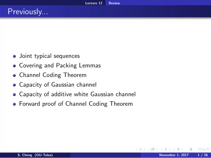
Lecture 12 Review Previously... Joint typical sequences Covering and Packing Lemmas Channel Coding Theorem Capacity of Gaussian channel Capacity of additive white Gaussian channel Forward proof of Channel Coding Theorem S. Cheng (OU-Tulsa)
Lecture 12 Capacity of non-white Gaussian channels Parallel Gaussian channels Consider that we have K parallel channels ( K bands) and the corresponding noise powers are σ 2 1 , σ 2 2 , · · · , σ 2 K S. Cheng (OU-Tulsa) November 1, 2017 7 / 26
Lecture 12 Capacity of non-white Gaussian channels Parallel Gaussian channels Consider that we have K parallel channels ( K bands) and the corresponding noise powers are σ 2 1 , σ 2 2 , · · · , σ 2 K And say, we can allocate a total of P power to all channels. The powers assigned to the channels are P 1 , P 2 , · · · , P K . So we need � K i =1 P i ≤ P S. Cheng (OU-Tulsa) November 1, 2017 7 / 26
Lecture 12 Capacity of non-white Gaussian channels Parallel Gaussian channels Consider that we have K parallel channels ( K bands) and the corresponding noise powers are σ 2 1 , σ 2 2 , · · · , σ 2 K And say, we can allocate a total of P power to all channels. The powers assigned to the channels are P 1 , P 2 , · · · , P K . So we need � K i =1 P i ≤ P � � Therefore, for the k -th channel, we can transmit 1 1 + P k 2 log bits σ 2 k per channel use S. Cheng (OU-Tulsa) November 1, 2017 7 / 26
Lecture 12 Capacity of non-white Gaussian channels Parallel Gaussian channels Consider that we have K parallel channels ( K bands) and the corresponding noise powers are σ 2 1 , σ 2 2 , · · · , σ 2 K And say, we can allocate a total of P power to all channels. The powers assigned to the channels are P 1 , P 2 , · · · , P K . So we need � K i =1 P i ≤ P � � Therefore, for the k -th channel, we can transmit 1 1 + P k 2 log bits σ 2 k per channel use So our goal is to assign P 1 , P 2 , · · · , P K ≥ 0 ( � K k =1 P k ≤ P ) such that the total capacity K � � 1 1 + P k � 2 log σ 2 k k =1 is maximize S. Cheng (OU-Tulsa) November 1, 2017 7 / 26
Lecture 12 Capacity of non-white Gaussian channels KKT conditions Let’s list all the KKT conditions for the optimization problem K 1 � � 1 + P k � max 2 log such that σ 2 k k =1 K � P 1 , · · · , P K ≥ 0 , P k ≤ P k =1 � K � K K �� ∂ 1 � 1 + P k � � � � λ k P k − µ P k − P 2 log + = 0 σ 2 ∂ P i k k =1 k =1 k =1 S. Cheng (OU-Tulsa) November 1, 2017 8 / 26
Lecture 12 Capacity of non-white Gaussian channels KKT conditions Let’s list all the KKT conditions for the optimization problem K 1 � � 1 + P k � max 2 log such that σ 2 k k =1 K � P 1 , · · · , P K ≥ 0 , P k ≤ P k =1 � K � K K �� ∂ 1 � 1 + P k � � � � λ k P k − µ P k − P 2 log + = 0 σ 2 ∂ P i k k =1 k =1 k =1 µ, λ 1 , · · · , λ K ≥ 0 S. Cheng (OU-Tulsa) November 1, 2017 8 / 26
Lecture 12 Capacity of non-white Gaussian channels KKT conditions Let’s list all the KKT conditions for the optimization problem K 1 � � 1 + P k � max 2 log such that σ 2 k k =1 K � P 1 , · · · , P K ≥ 0 , P k ≤ P k =1 � K � K K �� ∂ 1 � 1 + P k � � � � λ k P k − µ P k − P 2 log + = 0 σ 2 ∂ P i k k =1 k =1 k =1 K � µ, λ 1 , · · · , λ K ≥ 0 , P 1 , · · · , P K ≥ 0 , P k ≤ P k =1 S. Cheng (OU-Tulsa) November 1, 2017 8 / 26
Lecture 12 Capacity of non-white Gaussian channels KKT conditions Let’s list all the KKT conditions for the optimization problem K 1 � � 1 + P k � max 2 log such that σ 2 k k =1 K � P 1 , · · · , P K ≥ 0 , P k ≤ P k =1 � K � K K �� ∂ 1 � 1 + P k � � � � λ k P k − µ P k − P 2 log + = 0 σ 2 ∂ P i k k =1 k =1 k =1 K � µ, λ 1 , · · · , λ K ≥ 0 , P 1 , · · · , P K ≥ 0 , P k ≤ P k =1 � K � � µ P k − P = 0 , λ k P k = 0 , ∀ k k =1 S. Cheng (OU-Tulsa) November 1, 2017 8 / 26
Lecture 12 Capacity of non-white Gaussian channels Capacity of parallel channels � K � K K �� ∂ 1 � � 1 + P k � � � 2 log + λ k P k − µ P k − P = 0 σ 2 ∂ P i k k =1 k =1 k =1 S. Cheng (OU-Tulsa) November 1, 2017 9 / 26
Lecture 12 Capacity of non-white Gaussian channels Capacity of parallel channels � K � K K �� ∂ 1 � � 1 + P k � � � 2 log + λ k P k − µ P k − P = 0 σ 2 ∂ P i k k =1 k =1 k =1 ⇒ 1 1 = µ − λ i P i + σ 2 2 i S. Cheng (OU-Tulsa) November 1, 2017 9 / 26
Lecture 12 Capacity of non-white Gaussian channels Capacity of parallel channels � K � K K �� ∂ 1 � � 1 + P k � � � 2 log + λ k P k − µ P k − P = 0 σ 2 ∂ P i k k =1 k =1 k =1 ⇒ 1 1 1 = µ − λ i ⇒ P i + σ 2 i = P i + σ 2 2 2( µ − λ i ) i S. Cheng (OU-Tulsa) November 1, 2017 9 / 26
Lecture 12 Capacity of non-white Gaussian channels Capacity of parallel channels � K � K K �� ∂ 1 � � 1 + P k � � � 2 log + λ k P k − µ P k − P = 0 σ 2 ∂ P i k k =1 k =1 k =1 ⇒ 1 1 1 = µ − λ i ⇒ P i + σ 2 i = P i + σ 2 2 2( µ − λ i ) i Since λ i P i = 0, for P i > 0, we have λ i = 0 and thus i = 1 P i + σ 2 2 µ S. Cheng (OU-Tulsa) November 1, 2017 9 / 26
Lecture 12 Capacity of non-white Gaussian channels Capacity of parallel channels � K � K K �� ∂ 1 � � 1 + P k � � � 2 log + λ k P k − µ P k − P = 0 σ 2 ∂ P i k k =1 k =1 k =1 ⇒ 1 1 1 = µ − λ i ⇒ P i + σ 2 i = P i + σ 2 2 2( µ − λ i ) i Since λ i P i = 0, for P i > 0, we have λ i = 0 and thus i = 1 P i + σ 2 2 µ This suggests that µ > 0 and thus � K k =1 P k = P S. Cheng (OU-Tulsa) November 1, 2017 9 / 26
Lecture 12 Capacity of non-white Gaussian channels Capacity of parallel channels � K � K K �� ∂ 1 � � 1 + P k � � � 2 log + λ k P k − µ P k − P = 0 σ 2 ∂ P i k k =1 k =1 k =1 ⇒ 1 1 1 = µ − λ i ⇒ P i + σ 2 i = P i + σ 2 2 2( µ − λ i ) i Since λ i P i = 0, for P i > 0, we have λ i = 0 and thus i = 1 P i + σ 2 2 µ = constant This suggests that µ > 0 and thus � K k =1 P k = P S. Cheng (OU-Tulsa) November 1, 2017 9 / 26
Lecture 12 Capacity of non-white Gaussian channels Water-filling interpretation From P i + σ 2 i = const , power can be allocated intuitively as filling water to a pond (hence “water-filling”) Example S. Cheng (OU-Tulsa) November 1, 2017 10 / 26
Lecture 12 Capacity of non-white Gaussian channels Water-filling interpretation From P i + σ 2 i = const , power can be allocated intuitively as filling water to a pond (hence “water-filling”) Example P 1 = 0 , P 2 = 0 . 3 , P 3 = 0 . 6 , P 4 = 0 , P 5 = 0 S. Cheng (OU-Tulsa) November 1, 2017 10 / 26
Lecture 12 Capacity of non-white Gaussian channels Water-filling interpretation From P i + σ 2 i = const , power can be allocated intuitively as filling water to a pond (hence “water-filling”) Example P 1 = 0 , P 2 = 0 . 3 , P 3 = 0 . 6 , P 4 = 0 , P 5 = 0 P 1 = 0 , P 2 = 0 . 8 , P 3 = 1 . 1 , P 4 = 0 . 3 , P 5 = 0 S. Cheng (OU-Tulsa) November 1, 2017 10 / 26
Lecture 12 Capacity of non-white Gaussian channels Water-filling interpretation From P i + σ 2 i = const , power can be allocated intuitively as filling water to a pond (hence “water-filling”) Example P 1 = 0 , P 2 = 0 . 3 , P 3 = 0 . 6 , P 4 = 0 , P 5 = 0 P 1 = 0 , P 2 = 0 . 8 , P 3 = 1 . 1 , P 4 = 0 . 3 , P 5 = 0 P 1 = 0 . 5 , P 2 = 1 . 5 , P 3 = 1 . 8 , P 4 = 1 , P 5 = 0 S. Cheng (OU-Tulsa) November 1, 2017 10 / 26
Lecture 12 Capacity of non-white Gaussian channels Water-filling interpretation From P i + σ 2 i = const , power can be allocated intuitively as filling water to a pond (hence “water-filling”) Example P 1 = 0 , P 2 = 0 . 3 , P 3 = 0 . 6 , P 4 = 0 , P 5 = 0 P 1 = 0 , P 2 = 0 . 8 , P 3 = 1 . 1 , P 4 = 0 . 3 , P 5 = 0 P 1 = 0 . 5 , P 2 = 1 . 5 , P 3 = 1 . 8 , P 4 = 1 , P 5 = 0 S. Cheng (OU-Tulsa) November 1, 2017 10 / 26
Lecture 12 Rate-distortion problem Rate-distortion problem X N m p ( x ) ˆ Encoder Decoder X N We know that H ( X ) bits are needed on average to represent each sample of a source X S. Cheng (OU-Tulsa) November 1, 2017 11 / 26
Lecture 12 Rate-distortion problem Rate-distortion problem X N m p ( x ) ˆ Encoder Decoder X N We know that H ( X ) bits are needed on average to represent each sample of a source X If X is continuous, there is no way to recover X precisely S. Cheng (OU-Tulsa) November 1, 2017 11 / 26
Lecture 12 Rate-distortion problem Rate-distortion problem X N m p ( x ) ˆ Encoder Decoder X N We know that H ( X ) bits are needed on average to represent each sample of a source X If X is continuous, there is no way to recover X precisely Let say we are satisfied as long as we can recover X up to certain fidelity, how many bits are needed per sample? S. Cheng (OU-Tulsa) November 1, 2017 11 / 26
Lecture 12 Rate-distortion problem Rate-distortion problem X N m p ( x ) ˆ Encoder Decoder X N We know that H ( X ) bits are needed on average to represent each sample of a source X If X is continuous, there is no way to recover X precisely Let say we are satisfied as long as we can recover X up to certain fidelity, how many bits are needed per sample? There is an apparent rate (bits per sample) and distortion (fidelity) trade-off. We expect that needed rate is smaller if we allow a lower fidelity (higher distortion). What we are really interested in is a rate-distortion function S. Cheng (OU-Tulsa) November 1, 2017 11 / 26
Lecture 12 Rate-distortion problem Rate-distortion function m ∈ { 1 , 2 , · · · , M } X N m p ( x ) ˆ Encoder Decoder X N S. Cheng (OU-Tulsa) November 1, 2017 12 / 26
Lecture 12 Rate-distortion problem Rate-distortion function m ∈ { 1 , 2 , · · · , M } X N m p ( x ) ˆ Encoder Decoder X N N R = log M X N , X N )] = 1 D = E [ d ( ˆ � d ( ˆ , X i , X i ) N N i =1 S. Cheng (OU-Tulsa) November 1, 2017 12 / 26
Lecture 12 Rate-distortion problem Rate-distortion function m ∈ { 1 , 2 , · · · , M } X N m p ( x ) ˆ Encoder Decoder X N N R = log M X N , X N )] = 1 D = E [ d ( ˆ � d ( ˆ , X i , X i ) N N i =1 Maybe you can guess at this point. For given X and ˆ X , the required rate is simply I ( X ; ˆ X ) S. Cheng (OU-Tulsa) November 1, 2017 12 / 26
Lecture 12 Rate-distortion problem Rate-distortion function m ∈ { 1 , 2 , · · · , M } X N m p ( x ) ˆ Encoder Decoder X N N R = log M X N , X N )] = 1 D = E [ d ( ˆ � d ( ˆ , X i , X i ) N N i =1 Maybe you can guess at this point. For given X and ˆ X , the required rate is simply I ( X ; ˆ X ) How is it related to the distortion though? S. Cheng (OU-Tulsa) November 1, 2017 12 / 26
Lecture 12 Rate-distortion problem Rate-distortion function m ∈ { 1 , 2 , · · · , M } X N m p ( x ) ˆ Encoder Decoder X N N R = log M X N , X N )] = 1 D = E [ d ( ˆ � d ( ˆ , X i , X i ) N N i =1 Maybe you can guess at this point. For given X and ˆ X , the required rate is simply I ( X ; ˆ X ) How is it related to the distortion though? x | x ) such that E [ d ( ˆ X N , X N )] Note that we have a freedom to pick p (ˆ (less than or) equal to the desired D S. Cheng (OU-Tulsa) November 1, 2017 12 / 26
Lecture 12 Rate-distortion problem Rate-distortion function m ∈ { 1 , 2 , · · · , M } X N m p ( x ) ˆ Encoder Decoder X N N R = log M X N , X N )] = 1 D = E [ d ( ˆ � d ( ˆ , X i , X i ) N N i =1 Maybe you can guess at this point. For given X and ˆ X , the required rate is simply I ( X ; ˆ X ) How is it related to the distortion though? x | x ) such that E [ d ( ˆ X N , X N )] Note that we have a freedom to pick p (ˆ (less than or) equal to the desired D Therefore given D , the rate-distortion function is simply x | x ) I ( ˆ R ( D ) = min p (ˆ X ; X ) such that E [ d ( ˆ X N , X N )] ≤ D S. Cheng (OU-Tulsa) November 1, 2017 12 / 26
Lecture 12 Rate-distortion problem Binary symmetric source Let’s try to compress outcome from a fair coin toss S. Cheng (OU-Tulsa) November 1, 2017 13 / 26
Lecture 12 Rate-distortion problem Binary symmetric source Let’s try to compress outcome from a fair coin toss We know that we need 1 bit to compress the outcome losslessly, what if we have only 0.5 bit per sample? S. Cheng (OU-Tulsa) November 1, 2017 13 / 26
Lecture 12 Rate-distortion problem Binary symmetric source Let’s try to compress outcome from a fair coin toss We know that we need 1 bit to compress the outcome losslessly, what if we have only 0.5 bit per sample? In this case, we can’t losslessly recover the outcome. But how good will we do? S. Cheng (OU-Tulsa) November 1, 2017 13 / 26
Lecture 12 Rate-distortion problem Binary symmetric source Let’s try to compress outcome from a fair coin toss We know that we need 1 bit to compress the outcome losslessly, what if we have only 0.5 bit per sample? In this case, we can’t losslessly recover the outcome. But how good will we do? We need to introduce a distortion measure first. Note that we have two types of errors: taking head as tail and taking tail as head. A natural measure will just weights both error equally d ( X = H , ˆ X = T ) = d ( X = T , ˆ X = H ) = 1 d ( X = H , ˆ X = H ) = d ( X = T , ˆ X = T ) = 0 S. Cheng (OU-Tulsa) November 1, 2017 13 / 26
Lecture 12 Rate-distortion problem Binary symmetric source Let’s try to compress outcome from a fair coin toss We know that we need 1 bit to compress the outcome losslessly, what if we have only 0.5 bit per sample? In this case, we can’t losslessly recover the outcome. But how good will we do? We need to introduce a distortion measure first. Note that we have two types of errors: taking head as tail and taking tail as head. A natural measure will just weights both error equally d ( X = H , ˆ X = T ) = d ( X = T , ˆ X = H ) = 1 d ( X = H , ˆ X = H ) = d ( X = T , ˆ X = T ) = 0 If rate is > 1 bit, we know that distortion is 0. How about rate is 0, what distortion suppose to be? S. Cheng (OU-Tulsa) November 1, 2017 13 / 26
Lecture 12 Rate-distortion problem Binary symmetric source Let’s try to compress outcome from a fair coin toss We know that we need 1 bit to compress the outcome losslessly, what if we have only 0.5 bit per sample? In this case, we can’t losslessly recover the outcome. But how good will we do? We need to introduce a distortion measure first. Note that we have two types of errors: taking head as tail and taking tail as head. A natural measure will just weights both error equally d ( X = H , ˆ X = T ) = d ( X = T , ˆ X = H ) = 1 d ( X = H , ˆ X = H ) = d ( X = T , ˆ X = T ) = 0 If rate is > 1 bit, we know that distortion is 0. How about rate is 0, what distortion suppose to be? If decoders know nothing, the best bet will be just always decode head (or tail). Then D = E [ d ( X , H )] = 0 . 5 S. Cheng (OU-Tulsa) November 1, 2017 13 / 26
Lecture 12 Rate-distortion problem Binary symmetric source For 0 < D < 0 . 5, denote Z as the prediction error such that X = ˆ X + Z . S. Cheng (OU-Tulsa) November 1, 2017 14 / 26
Lecture 12 Rate-distortion problem Binary symmetric source For 0 < D < 0 . 5, denote Z as the prediction error such that X = ˆ X + Z . Note that Pr ( Z = 1) = D S. Cheng (OU-Tulsa) November 1, 2017 14 / 26
Lecture 12 Rate-distortion problem Binary symmetric source For 0 < D < 0 . 5, denote Z as the prediction error such that X = ˆ X + Z . Note that Pr ( Z = 1) = D x | x ) I ( ˆ x | x ) H ( X ) − H ( X | ˆ R = min p (ˆ X ; X ) = min p (ˆ X ) S. Cheng (OU-Tulsa) November 1, 2017 14 / 26
Lecture 12 Rate-distortion problem Binary symmetric source For 0 < D < 0 . 5, denote Z as the prediction error such that X = ˆ X + Z . Note that Pr ( Z = 1) = D x | x ) I ( ˆ x | x ) H ( X ) − H ( X | ˆ R = min p (ˆ X ; X ) = min p (ˆ X ) x | x ) H ( X ) − H ( ˆ X + Z | ˆ = min p (ˆ X ) S. Cheng (OU-Tulsa) November 1, 2017 14 / 26
Lecture 12 Rate-distortion problem Binary symmetric source For 0 < D < 0 . 5, denote Z as the prediction error such that X = ˆ X + Z . Note that Pr ( Z = 1) = D x | x ) I ( ˆ x | x ) H ( X ) − H ( X | ˆ R = min p (ˆ X ; X ) = min p (ˆ X ) x | x ) H ( X ) − H ( ˆ X + Z | ˆ = min p (ˆ X ) x | x ) H ( X ) − H ( Z | ˆ = min p (ˆ X ) S. Cheng (OU-Tulsa) November 1, 2017 14 / 26
Lecture 12 Rate-distortion problem Binary symmetric source For 0 < D < 0 . 5, denote Z as the prediction error such that X = ˆ X + Z . Note that Pr ( Z = 1) = D x | x ) I ( ˆ x | x ) H ( X ) − H ( X | ˆ R = min p (ˆ X ; X ) = min p (ˆ X ) x | x ) H ( X ) − H ( ˆ X + Z | ˆ = min p (ˆ X ) x | x ) H ( X ) − H ( Z | ˆ = min p (ˆ X ) x | x ) H ( X ) − H ( Z ) = min p (ˆ S. Cheng (OU-Tulsa) November 1, 2017 14 / 26
Lecture 12 Rate-distortion problem Binary symmetric source For 0 < D < 0 . 5, denote Z as the prediction error such that X = ˆ X + Z . Note that Pr ( Z = 1) = D x | x ) I ( ˆ x | x ) H ( X ) − H ( X | ˆ R = min p (ˆ X ; X ) = min p (ˆ X ) x | x ) H ( X ) − H ( ˆ X + Z | ˆ = min p (ˆ X ) 1 x | x ) H ( X ) − H ( Z | ˆ = min p (ˆ X ) 0 . 8 x | x ) H ( X ) − H ( Z ) = min p (ˆ 0 . 6 R ( D ) 0 . 4 = 1 − H ( D ) 0 . 2 D 0 . 1 0 . 2 0 . 3 0 . 4 0 . 5 S. Cheng (OU-Tulsa) November 1, 2017 14 / 26
Lecture 12 Rate-distortion problem Gaussian source Consider X ∼ N (0 , σ 2 X ). To determine the rate-distortion function, we need first to decide the distortion measure. An intuitive will be just the square error. That is, d ( ˆ X , X ) = ( ˆ X − X ) 2 S. Cheng (OU-Tulsa) November 1, 2017 15 / 26
Lecture 12 Rate-distortion problem Gaussian source Consider X ∼ N (0 , σ 2 X ). To determine the rate-distortion function, we need first to decide the distortion measure. An intuitive will be just the square error. That is, d ( ˆ X , X ) = ( ˆ X − X ) 2 Given E [ d ( ˆ X , X )] = D , what is the minimum rate required? S. Cheng (OU-Tulsa) November 1, 2017 15 / 26
Lecture 12 Rate-distortion problem Gaussian source Consider X ∼ N (0 , σ 2 X ). To determine the rate-distortion function, we need first to decide the distortion measure. An intuitive will be just the square error. That is, d ( ˆ X , X ) = ( ˆ X − X ) 2 Given E [ d ( ˆ X , X )] = D , what is the minimum rate required? Like before, let us denote Z = X − ˆ X as the prediction error. Note that Var ( Z ) = D S. Cheng (OU-Tulsa) November 1, 2017 15 / 26
Lecture 12 Rate-distortion problem Gaussian source Consider X ∼ N (0 , σ 2 X ). To determine the rate-distortion function, we need first to decide the distortion measure. An intuitive will be just the square error. That is, d ( ˆ X , X ) = ( ˆ X − X ) 2 Given E [ d ( ˆ X , X )] = D , what is the minimum rate required? Like before, let us denote Z = X − ˆ X as the prediction error. Note that Var ( Z ) = D x | x ) I ( ˆ x | x ) h ( X ) − h ( X | ˆ R ( D ) = min p (ˆ X ; X ) = min p (ˆ X ) S. Cheng (OU-Tulsa) November 1, 2017 15 / 26
Lecture 12 Rate-distortion problem Gaussian source Consider X ∼ N (0 , σ 2 X ). To determine the rate-distortion function, we need first to decide the distortion measure. An intuitive will be just the square error. That is, d ( ˆ X , X ) = ( ˆ X − X ) 2 Given E [ d ( ˆ X , X )] = D , what is the minimum rate required? Like before, let us denote Z = X − ˆ X as the prediction error. Note that Var ( Z ) = D x | x ) I ( ˆ x | x ) h ( X ) − h ( X | ˆ R ( D ) = min p (ˆ X ; X ) = min p (ˆ X ) x | x ) h ( X ) − h ( Z + ˆ X | ˆ = min p (ˆ X ) S. Cheng (OU-Tulsa) November 1, 2017 15 / 26
Lecture 12 Rate-distortion problem Gaussian source Consider X ∼ N (0 , σ 2 X ). To determine the rate-distortion function, we need first to decide the distortion measure. An intuitive will be just the square error. That is, d ( ˆ X , X ) = ( ˆ X − X ) 2 Given E [ d ( ˆ X , X )] = D , what is the minimum rate required? Like before, let us denote Z = X − ˆ X as the prediction error. Note that Var ( Z ) = D x | x ) I ( ˆ x | x ) h ( X ) − h ( X | ˆ R ( D ) = min p (ˆ X ; X ) = min p (ˆ X ) x | x ) h ( X ) − h ( Z + ˆ X | ˆ = min p (ˆ X ) x | x ) h ( X ) − h ( Z | ˆ = min p (ˆ X ) S. Cheng (OU-Tulsa) November 1, 2017 15 / 26
Lecture 12 Rate-distortion problem Gaussian source Consider X ∼ N (0 , σ 2 X ). To determine the rate-distortion function, we need first to decide the distortion measure. An intuitive will be just the square error. That is, d ( ˆ X , X ) = ( ˆ X − X ) 2 Given E [ d ( ˆ X , X )] = D , what is the minimum rate required? Like before, let us denote Z = X − ˆ X as the prediction error. Note that Var ( Z ) = D x | x ) I ( ˆ x | x ) h ( X ) − h ( X | ˆ R ( D ) = min p (ˆ X ; X ) = min p (ˆ X ) x | x ) h ( X ) − h ( Z + ˆ X | ˆ = min p (ˆ X ) x | x ) h ( X ) − h ( Z | ˆ = min p (ˆ X ) = min p (ˆ x | x ) h ( X ) − h ( Z ) S. Cheng (OU-Tulsa) November 1, 2017 15 / 26
Lecture 12 Rate-distortion problem Gaussian source Consider X ∼ N (0 , σ 2 X ). To determine the rate-distortion function, we need first to decide the distortion measure. An intuitive will be just the square error. That is, d ( ˆ X , X ) = ( ˆ X − X ) 2 Given E [ d ( ˆ X , X )] = D , what is the minimum rate required? Like before, let us denote Z = X − ˆ X as the prediction error. Note that Var ( Z ) = D x | x ) I ( ˆ x | x ) h ( X ) − h ( X | ˆ R ( D ) = min p (ˆ X ; X ) = min p (ˆ X ) x | x ) h ( X ) − h ( Z + ˆ X | ˆ = min p (ˆ X ) x | x ) h ( X ) − h ( Z | ˆ = min p (ˆ X ) = min p (ˆ x | x ) h ( X ) − h ( Z ) = log σ 2 X D S. Cheng (OU-Tulsa) November 1, 2017 15 / 26
Lecture 12 Rate-distortion Theorem Forward proof Forward statement Given distortion constraint D , we can find scheme such that the require rate is no bigger than x | x ) I ( X ; ˆ R ( D ) = min X ) , p (ˆ where the ˆ x | x ) should satisfy E [ d ( X , ˆ X introduced by p (ˆ X )] ≤ D S. Cheng (OU-Tulsa) November 1, 2017 16 / 26
Lecture 12 Rate-distortion Theorem Forward proof Forward statement Given distortion constraint D , we can find scheme such that the require rate is no bigger than x | x ) I ( X ; ˆ R ( D ) = min X ) , p (ˆ where the ˆ x | x ) should satisfy E [ d ( X , ˆ X introduced by p (ˆ X )] ≤ D Code book construction Let say p ∗ (ˆ x | x ) is the distribution that achieve the rate-distortion optimiation problem. Randomly construct 2 NR codewords as follows S. Cheng (OU-Tulsa) November 1, 2017 16 / 26
Lecture 12 Rate-distortion Theorem Forward proof Forward statement Given distortion constraint D , we can find scheme such that the require rate is no bigger than x | x ) I ( X ; ˆ R ( D ) = min X ) , p (ˆ where the ˆ x | x ) should satisfy E [ d ( X , ˆ X introduced by p (ˆ X )] ≤ D Code book construction Let say p ∗ (ˆ x | x ) is the distribution that achieve the rate-distortion optimiation problem. Randomly construct 2 NR codewords as follows x | x ) to obtain ˆ Sample X from the source and pass X into p ∗ (ˆ X S. Cheng (OU-Tulsa) November 1, 2017 16 / 26
Lecture 12 Rate-distortion Theorem Forward proof Forward statement Given distortion constraint D , we can find scheme such that the require rate is no bigger than x | x ) I ( X ; ˆ R ( D ) = min X ) , p (ˆ where the ˆ x | x ) should satisfy E [ d ( X , ˆ X introduced by p (ˆ X )] ≤ D Code book construction Let say p ∗ (ˆ x | x ) is the distribution that achieve the rate-distortion optimiation problem. Randomly construct 2 NR codewords as follows x | x ) to obtain ˆ Sample X from the source and pass X into p ∗ (ˆ X Repeat this N time to get a length- N codeword Store the i -th codeword as C ( i ) S. Cheng (OU-Tulsa) November 1, 2017 16 / 26
Lecture 12 Rate-distortion Theorem Forward proof Forward statement Given distortion constraint D , we can find scheme such that the require rate is no bigger than x | x ) I ( X ; ˆ R ( D ) = min X ) , p (ˆ where the ˆ x | x ) should satisfy E [ d ( X , ˆ X introduced by p (ˆ X )] ≤ D Code book construction Let say p ∗ (ˆ x | x ) is the distribution that achieve the rate-distortion optimiation problem. Randomly construct 2 NR codewords as follows x | x ) to obtain ˆ Sample X from the source and pass X into p ∗ (ˆ X Repeat this N time to get a length- N codeword Store the i -th codeword as C ( i ) Note that the code rate is log 2 NR = R as desired N S. Cheng (OU-Tulsa) November 1, 2017 16 / 26
Lecture 12 Rate-distortion Theorem Covering lemma and distortion typical sequences We say joint typical sequences x N and ˆ x N are distortion typical x N ) − E [ d ( X , ˆ (( x N , ˆ x N ) ∈ A N d ,ǫ ) if | d ( x N , ˆ X )] | ≤ ǫ S. Cheng (OU-Tulsa) November 1, 2017 17 / 26
Lecture 12 Rate-distortion Theorem Covering lemma and distortion typical sequences We say joint typical sequences x N and ˆ x N are distortion typical x N ) − E [ d ( X , ˆ (( x N , ˆ x N ) ∈ A N d ,ǫ ) if | d ( x N , ˆ X )] | ≤ ǫ By LLN, every pair of sequences sampled from the joint source will virtually be distortion typical S. Cheng (OU-Tulsa) November 1, 2017 17 / 26
Lecture 12 Rate-distortion Theorem Covering lemma and distortion typical sequences We say joint typical sequences x N and ˆ x N are distortion typical x N ) − E [ d ( X , ˆ (( x N , ˆ x N ) ∈ A N d ,ǫ ) if | d ( x N , ˆ X )] | ≤ ǫ By LLN, every pair of sequences sampled from the joint source will virtually be distortion typical X ) − ǫ ) ≤ |A N Consequently, (1 − δ )2 N ( H ( X , ˆ d ,ǫ | ≤ 2 N ( H ( X , ˆ X )+ ǫ ) as before S. Cheng (OU-Tulsa) November 1, 2017 17 / 26
Lecture 12 Rate-distortion Theorem Covering lemma and distortion typical sequences We say joint typical sequences x N and ˆ x N are distortion typical x N ) − E [ d ( X , ˆ (( x N , ˆ x N ) ∈ A N d ,ǫ ) if | d ( x N , ˆ X )] | ≤ ǫ By LLN, every pair of sequences sampled from the joint source will virtually be distortion typical X ) − ǫ ) ≤ |A N Consequently, (1 − δ )2 N ( H ( X , ˆ d ,ǫ | ≤ 2 N ( H ( X , ˆ X )+ ǫ ) as before X N and X N , the probability For two independently drawn sequences ˆ for them to be distortion typical will be just the same as before. In particular, (1 − δ )2 − N ( I ( X ; ˆ X ) − 3 ǫ ) ≤ Pr (( X N , ˆ d ,ǫ ( X , ˆ X N ) ∈ A N X )) S. Cheng (OU-Tulsa) November 1, 2017 17 / 26
Lecture 12 Rate-distortion Theorem Covering lemma for distortion typical sequences S. Cheng (OU-Tulsa) November 1, 2017 18 / 26
Lecture 12 Rate-distortion Theorem Covering lemma for distortion typical sequences ∈ A ( N ) Pr (( X N ( m ) , ˆ X N ) / d ,ǫ ( X , ˆ X ) for all m ) S. Cheng (OU-Tulsa) November 1, 2017 18 / 26
Lecture 12 Rate-distortion Theorem Covering lemma for distortion typical sequences ∈ A ( N ) Pr (( X N ( m ) , ˆ X N ) / d ,ǫ ( X , ˆ X ) for all m ) M ∈ A ( N ) � Pr (( X N ( m ) , ˆ d ,ǫ ( ˆ X N ) / = X , X )) m =1 S. Cheng (OU-Tulsa) November 1, 2017 18 / 26
Lecture 12 Rate-distortion Theorem Covering lemma for distortion typical sequences ∈ A ( N ) Pr (( X N ( m ) , ˆ X N ) / d ,ǫ ( X , ˆ X ) for all m ) M ∈ A ( N ) � Pr (( X N ( m ) , ˆ d ,ǫ ( ˆ X N ) / = X , X )) m =1 M � X N ) ∈ A ( N ) � � 1 − Pr (( X N ( m ) , ˆ d ,ǫ ( ˆ = X , X )) m =1 S. Cheng (OU-Tulsa) November 1, 2017 18 / 26
Lecture 12 Rate-distortion Theorem Covering lemma for distortion typical sequences ∈ A ( N ) Pr (( X N ( m ) , ˆ X N ) / d ,ǫ ( X , ˆ X ) for all m ) M ∈ A ( N ) � Pr (( X N ( m ) , ˆ d ,ǫ ( ˆ X N ) / = X , X )) m =1 M � X N ) ∈ A ( N ) � � 1 − Pr (( X N ( m ) , ˆ d ,ǫ ( ˆ = X , X )) m =1 ≤ (1 − (1 − δ )2 − N ( I ( ˆ X ; X )+3 ǫ ) ) M S. Cheng (OU-Tulsa) November 1, 2017 18 / 26
Lecture 12 Rate-distortion Theorem Covering lemma for distortion typical sequences ∈ A ( N ) Pr (( X N ( m ) , ˆ X N ) / d ,ǫ ( X , ˆ X ) for all m ) 0 M ∈ A ( N ) � Pr (( X N ( m ) , ˆ d ,ǫ ( ˆ X N ) / = X , X )) − 2 m =1 M − 4 � X N ) ∈ A ( N ) � � 1 − Pr (( X N ( m ) , ˆ d ,ǫ ( ˆ = X , X )) 0 2 4 m =1 1 − x ≤ (1 − (1 − δ )2 − N ( I ( ˆ X ; X )+3 ǫ ) ) M e − x ≤ exp( − M (1 − δ )2 − N ( I ( ˆ X ; X )+3 ǫ ) ) S. Cheng (OU-Tulsa) November 1, 2017 18 / 26
Lecture 12 Rate-distortion Theorem Covering lemma for distortion typical sequences ∈ A ( N ) Pr (( X N ( m ) , ˆ X N ) / d ,ǫ ( X , ˆ X ) for all m ) 0 M ∈ A ( N ) � Pr (( X N ( m ) , ˆ d ,ǫ ( ˆ X N ) / = X , X )) − 2 m =1 M − 4 � X N ) ∈ A ( N ) � � 1 − Pr (( X N ( m ) , ˆ d ,ǫ ( ˆ = X , X )) 0 2 4 m =1 1 − x ≤ (1 − (1 − δ )2 − N ( I ( ˆ X ; X )+3 ǫ ) ) M e − x ≤ exp( − M (1 − δ )2 − N ( I ( ˆ X ; X )+3 ǫ ) ) ≤ exp( − (1 − δ )2 − N ( I ( ˆ X ; X ) − R +3 ǫ ) ) → 0 as N → ∞ and R > I ( X ; ˆ X ) S. Cheng (OU-Tulsa) November 1, 2017 18 / 26
Lecture 12 Rate-distortion Theorem Forward proof Encoding Given input X N , find out of the codewords the one that is jointly typical with X N . And say, if the codeword is C ( i ), output index i to the decoder S. Cheng (OU-Tulsa) November 1, 2017 19 / 26
Lecture 12 Rate-distortion Theorem Forward proof Encoding Given input X N , find out of the codewords the one that is jointly typical with X N . And say, if the codeword is C ( i ), output index i to the decoder Decoding Upon receiving the index i , simply output C ( i ) S. Cheng (OU-Tulsa) November 1, 2017 19 / 26
Lecture 12 Rate-distortion Theorem Forward proof Encoding Given input X N , find out of the codewords the one that is jointly typical with X N . And say, if the codeword is C ( i ), output index i to the decoder Decoding Upon receiving the index i , simply output C ( i ) Performance analysis First of all, the only point of failure lies on encoding, that is when the encoder cannot find a codeword jointly typical with X N S. Cheng (OU-Tulsa) November 1, 2017 19 / 26
Lecture 12 Rate-distortion Theorem Forward proof Encoding Given input X N , find out of the codewords the one that is jointly typical with X N . And say, if the codeword is C ( i ), output index i to the decoder Decoding Upon receiving the index i , simply output C ( i ) Performance analysis First of all, the only point of failure lies on encoding, that is when the encoder cannot find a codeword jointly typical with X N By covering Lemma, encoding failure is neglible as long as R > I ( X ; ˆ X ) S. Cheng (OU-Tulsa) November 1, 2017 19 / 26
Lecture 12 Rate-distortion Theorem Forward proof Encoding Given input X N , find out of the codewords the one that is jointly typical with X N . And say, if the codeword is C ( i ), output index i to the decoder Decoding Upon receiving the index i , simply output C ( i ) Performance analysis First of all, the only point of failure lies on encoding, that is when the encoder cannot find a codeword jointly typical with X N By covering Lemma, encoding failure is neglible as long as R > I ( X ; ˆ X ) If encoding is successful, C ( i ) and X N should be distortion typical. Therefore, E [ d ( C ( i ); X N )] ∼ E [ d ( ˆ X , X )] ≤ D as desired S. Cheng (OU-Tulsa) November 1, 2017 19 / 26
Lecture 12 Rate-distortion Theorem Converse proof Converse statement If rate is smaller than R ( D ), distortion will be larger than D S. Cheng (OU-Tulsa) November 1, 2017 20 / 26
Lecture 12 Rate-distortion Theorem Converse proof Converse statement If rate is smaller than R ( D ), distortion will be larger than D Alternative statement If distortion is less than or equal to D , the rate must be larger than R ( D ) S. Cheng (OU-Tulsa) November 1, 2017 20 / 26
Lecture 12 Rate-distortion Theorem Converse proof Converse statement If rate is smaller than R ( D ), distortion will be larger than D Alternative statement If distortion is less than or equal to D , the rate must be larger than R ( D ) In the proof, we need to use the convex property of R ( D ). That is, R ( a D 1 + (1 − a ) D 2 ) ≥ aR ( D 1 ) + (1 − a ) R ( D 2 ) So we will digress a little bit to show this convex property first S. Cheng (OU-Tulsa) November 1, 2017 20 / 26
Lecture 12 Rate-distortion Theorem Log-sum inequality Log-sum inequality For any a 1 , · · · , a n ≥ 0 and b 1 , · · · , b n ≥ 0, we have � a i i a i � � a i log 2 ≥ a i log 2 . � b i i b i i i S. Cheng (OU-Tulsa) November 1, 2017 21 / 26
Lecture 12 Rate-distortion Theorem Log-sum inequality Log-sum inequality For any a 1 , · · · , a n ≥ 0 and b 1 , · · · , b n ≥ 0, we have � a i i a i � � a i log 2 ≥ a i log 2 . � b i i b i i i Proof a i We can define two distributions p ( x ) and q ( x ) with p ( x i ) = i a i and � b i q ( x i ) = i b i . Since p ( x ) and q ( x ) are both non-negative and sum up to � 1, they are indeed valid probability mass functions. S. Cheng (OU-Tulsa) November 1, 2017 21 / 26
Recommend
More recommend
Explore More Topics
Stay informed with curated content and fresh updates.


