Preliminary version THE VALIDITY OF PURCHASING POWER PARITY THEORY - PDF document
Preliminary version THE VALIDITY OF PURCHASING POWER PARITY THEORY IN TRANSITION Darja Bori University of Maribor, Slovenia INTRODUCTION The theory of purchasing power parity became particularly interesting after the introduction of
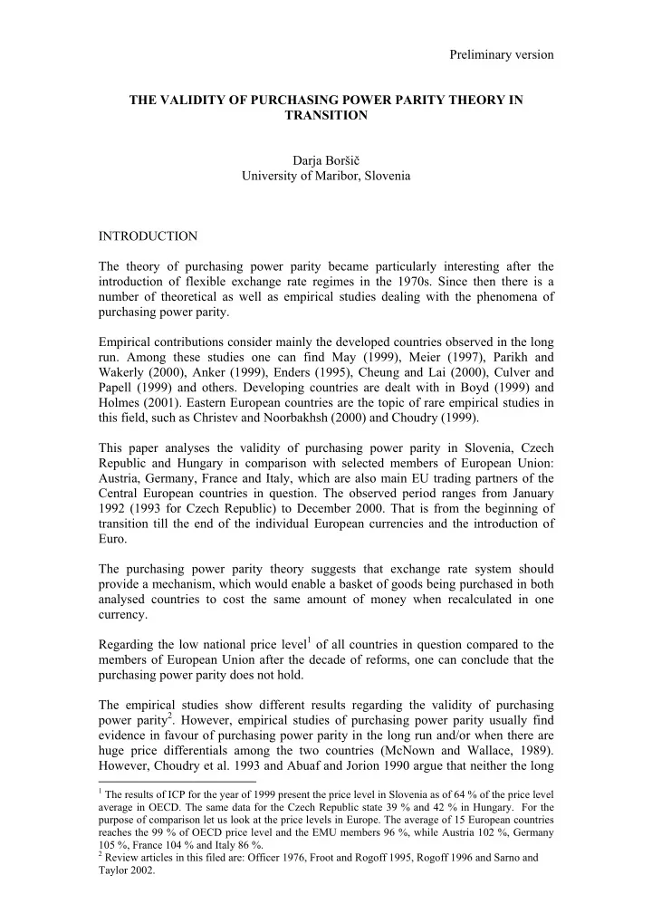
Preliminary version THE VALIDITY OF PURCHASING POWER PARITY THEORY IN TRANSITION Darja Borši č University of Maribor, Slovenia INTRODUCTION The theory of purchasing power parity became particularly interesting after the introduction of flexible exchange rate regimes in the 1970s. Since then there is a number of theoretical as well as empirical studies dealing with the phenomena of purchasing power parity. Empirical contributions consider mainly the developed countries observed in the long run. Among these studies one can find May (1999), Meier (1997), Parikh and Wakerly (2000), Anker (1999), Enders (1995), Cheung and Lai (2000), Culver and Papell (1999) and others. Developing countries are dealt with in Boyd (1999) and Holmes (2001). Eastern European countries are the topic of rare empirical studies in this field, such as Christev and Noorbakhsh (2000) and Choudry (1999). This paper analyses the validity of purchasing power parity in Slovenia, Czech Republic and Hungary in comparison with selected members of European Union: Austria, Germany, France and Italy, which are also main EU trading partners of the Central European countries in question. The observed period ranges from January 1992 (1993 for Czech Republic) to December 2000. That is from the beginning of transition till the end of the individual European currencies and the introduction of Euro. The purchasing power parity theory suggests that exchange rate system should provide a mechanism, which would enable a basket of goods being purchased in both analysed countries to cost the same amount of money when recalculated in one currency. Regarding the low national price level 1 of all countries in question compared to the members of European Union after the decade of reforms, one can conclude that the purchasing power parity does not hold. The empirical studies show different results regarding the validity of purchasing power parity 2 . However, empirical studies of purchasing power parity usually find evidence in favour of purchasing power parity in the long run and/or when there are huge price differentials among the two countries (McNown and Wallace, 1989). However, Choudry et al. 1993 and Abuaf and Jorion 1990 argue that neither the long 1 The results of ICP for the year of 1999 present the price level in Slovenia as of 64 % of the price level average in OECD. The same data for the Czech Republic state 39 % and 42 % in Hungary. For the purpose of comparison let us look at the price levels in Europe. The average of 15 European countries reaches the 99 % of OECD price level and the EMU members 96 %, while Austria 102 %, Germany 105 %, France 104 % and Italy 86 %. 2 Review articles in this filed are: Officer 1976, Froot and Rogoff 1995, Rogoff 1996 and Sarno and Taylor 2002.
run nor the high inflation is not the sufficient condition for the validity of purchasing power parity. The analyses proving the validity of this theory in the periods of high inflation include Frenkel (1978), Taylor and McMahon (1988), McNown and Wallace (1989) and Liu (1992). Consequently, there is a chance that the hypothesis of this paper could be rejected due to the periods of relatively high inflation in the observed Central European countries in the beginning of the transition period. Since the observed Central European countries are all suppose to became full members of EU in the near future, the purchasing power parity and the price level should gradually converge to the European average. Thus, this study can contribute to the recognition and understanding of the present differences in the purchasing power parity and price levels among the Central European countries and their main EU trading partners. THEORY OF PURCHASING POWER PARITY The absolute purchasing power parity According to the theory of purchasing power parity the exchange rate among two countries should be equal to the price level of the observed economies. For each basket of goods the exchange rate is suppose to provide the mechanism enabling to buy the same basket of goods abroad for the same price as at home. Thus, the absolute version of the theory applies that the exchange rates and the national price levels constitute an equilibrium relation ship, which can be presented as follows. e t = α 0 + α 1 p t + ξ t (1), where e t is the logarithm of nominal exchange rate measured in the units of domestic currency needed for a unit of foreign currency, p t is the logarithm of price ratio and ξ t is the residual. The relative purchasing power parity The relative version of the theory applies that relative change in exchange rate equals the relative change in price level in the two observed economies. This version of purchasing power parity actually suggests that exchange rate fluctuations eliminate the price differences among the two countries. If E t presents the nominal exchange rate, P t indicates price index and * a foreign country, the relative version of the purchasing power parity can be expressed as below: * E P P = − t t t 1 (2) * E P P t - 1 t − 1 t Price indices show the costs of a basket of goods in the observed time period compared to a base point in time. Increased price indices are a sign of inflation, indicating that relative costs of the same basket of goods increased. Consumer price index and producer price index are the most common price indices, the later presenting tradables prices, while the former reflecting also the prices of non tradable goods. However, the methodology of the price recording varies from a country to a country, resulting in specific baskets of goods in national price indices and disabling a
proper comparison of prices among the economies. Here the relative version of the theory has an advantage since it deals with the changes in price indices and exchange rates and not with their absolute figures. TESTING FOR THE PURCHASING POWER PARITY IN TRANSITION The general model of testing for purchasing power parity (Cheung and Lai 1993) is the following: e t = α 0 + α 1 P t - α 2 P t * + ξ t (3), where e t stands for nominal exchange rates, presented as the price of foreign currency in the units of domestic currency, P are domestic prices and P* are foreign prices. All the variables are in the logarithmic form. In the most restrictive form, there are the following restrictions: α 0 = 0, α 1 = α 2 =1. The symmetry restriction applies that α 1 and α 2 are equal, while the limitation of α 1 and α 2 being equal to one is called the proportionality restriction (Froot in Rogoff 1995). Testing the real exchange rates The empirical analysis starts off with the most restrictive version of the model ( α 1 = α 2 =1), that is testing the real exchange rates. In the context of the relative PPP the movements in exchange rates are expected to compensate for price level shifts. Thus, real exchange rates should be constant over a long run and their time series should be stationary. The real exchange rates are calculated from the nominal exchange rates using the consumer price index (CPI), which includes the whole range of price, the tradables as well as the non tradables: re t = e t + p t * - p t (4), where re t stands for the real exchange rate, e t is the price of a foreign currency in units of domestic currency , p are consumer price indices and * indicates a foreign country. In this way, the real exchange rates are calculated for Slovene tolar, Hungarian forint and the Czech koruna regarding Austria, Germany, France and Italy. The stationarity of real exchange rates is first being checked graphically and then confirmed by Augmented Dickey Fuller test. Time series are stationary if their mean and variance are constant over time, while the value of the covariance depends only on the time lag and not on the actual time point where the covariance is being calculated. Enders (1995) argues that the shocks to which a stationary time series is exposed to are temporary and their influence gradually diminish. Consequently, the time series converges to its long run mean. The covariance of a stationary time series converges to its mean and fluctuates around its constant long run mean, the variance of the series does not depend on a time lag and its correlogram disappears while the time lag increase. On the contrary, the mean and the variance of a nonstationary time series depend on the time lag, there is no long run mean to which the series would converge, the variance depends on the time lag and its value increases while the time lag increases, its correlogram does not diminish quickly but slowly decreases.
Recommend
More recommend
Explore More Topics
Stay informed with curated content and fresh updates.
