Predicting a New Response Recall the regression model y = 0 + 1 x - PowerPoint PPT Presentation

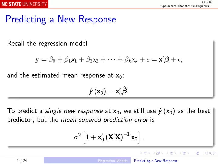
ST 516 Experimental Statistics for Engineers II Predicting a New Response Recall the regression model y = β 0 + β 1 x 1 + β 2 x 2 + · · · + β k x k + ǫ = x ′ β + ǫ, and the estimated mean response at x 0 : 0 ˆ y ( x 0 ) = x ′ ˆ β . To predict a single new response at x 0 , we still use ˆ y ( x 0 ) as the best predictor, but the mean squared prediction error is 0 ( X ′ X ) − 1 x 0 σ 2 � � 1 + x ′ . 1 / 24 Regression Models Predicting a New Response

ST 516 Experimental Statistics for Engineers II So the 100(1 − α )% prediction interval is � 0 ( X ′ X ) − 1 x 0 � � y ( x 0 ) ± t α/ 2 , n − p ˆ σ 2 ˆ 1 + x ′ Note that this is wider than the 100(1 − α )% confidence interval for the mean response at x 0 , � 0 ( X ′ X ) − 1 x 0 σ 2 x ′ y ( x 0 ) ± t α/ 2 , n − p ˆ ˆ because the prediction interval must allow for the ǫ in the new response: new response = mean response + ǫ. 2 / 24 Regression Models Predicting a New Response

ST 516 Experimental Statistics for Engineers II R command Use predict(..., interval = "prediction") : predict(viscosityLm, newdata = data.frame(Temperature = 90, CatalystFeedRate = 10), se.fit = TRUE, interval = "prediction") Output $fit fit lwr upr 1 2337.842 2301.360 2374.325 $se.fit [1] 4.192114 $df [1] 13 $residual.scale [1] 16.35860 3 / 24 Regression Models Predicting a New Response

ST 516 Experimental Statistics for Engineers II The prediction interval is centered at the same value of fit as the confidence interval. The prediction interval is wider than the confidence interval, because of the variability in a single observation. Both of these intervals used the default confidence/prediction level of 95%; use predict(..., level = .99) , for instance, to change the level. 4 / 24 Regression Models Predicting a New Response

ST 516 Experimental Statistics for Engineers II Regression Diagnostics Standard residual plots are: Qq-plot (probability plot) of residuals; Plot residuals against fitted values; Plot residuals against regressors; Plot (square roots of) absolute residuals against fitted values. More diagnostics are usually examined after a regression analysis. 5 / 24 Regression Models Regression Diagnostics

ST 516 Experimental Statistics for Engineers II Scaled Residuals Residuals are usually scaled in various ways. E.g. the standardized residual e i d i = √ σ 2 , ˆ is dimensionless; they satisfy n � d i = 0 i =1 and n � d 2 i = n − p . i =1 6 / 24 Regression Models Regression Diagnostics

ST 516 Experimental Statistics for Engineers II The d i are therefore “standardized” in an average sense. But the standard deviation of the i th residual e i usually depends on i . So the d i are not individually standardized. 7 / 24 Regression Models Regression Diagnostics

ST 516 Experimental Statistics for Engineers II The hat matrix: y = X ˆ ˆ β = X ( X ′ X ) − 1 X ′ y = Hy where H = X ( X ′ X ) − 1 X ′ is the hat matrix (so called because it “puts the hat on y ”). So the residuals e satisfy e = y − ˆ y = ( I − H ) y and Cov( e ) = σ 2 ( I − H ) . 8 / 24 Regression Models Regression Diagnostics

ST 516 Experimental Statistics for Engineers II So the variance of the i th residual is V( e i ) = σ 2 (1 − h i , i ) where h i , i is the i th diagonal entry of H . The studentized residual is e i d i r i = = σ 2 (1 − h i , i ) � � ˆ (1 − h i , i ) with population mean 0 and variance 1 for each i : E( r i ) = 0 , V( r i ) = 1 . 9 / 24 Regression Models Regression Diagnostics

ST 516 Experimental Statistics for Engineers II Cross Validation Suppose we predict y i from a data set excluding y i . New parameter estimates ˆ β ( i ) . i ˆ Predicted value is ˆ y ( i ) = x ′ β ( i ) and the corresponding residual satisfies e i e ( i ) = y i − ˆ y ( i ) = . 1 − h i , i The PRediction Error Sum of Squares statistic (PRESS) is n � e 2 PRESS = ( i ) . i =1 10 / 24 Regression Models Regression Diagnostics

ST 516 Experimental Statistics for Engineers II Approximate R 2 for prediction: prediction = 1 − PRESS R 2 . SS T E.g. for viscosity example, PRESS = 5207 . 7, so R 2 prediction = . 891. Recall R 2 = . 927 and R 2 adj = . 916: R 2 prediction penalizes over-fitting more than does R 2 adj . 11 / 24 Regression Models Regression Diagnostics

ST 516 Experimental Statistics for Engineers II R function RsqPred <- function(l) { infl <- influence(l) PRESS <- sum((infl$wt.res / (1 - infl$hat))^2) rsq <- summary(l)$r.squared sst <- sum(infl$wt.res^2) / (1 - rsq) 1 - PRESS / sst } RsqPred(lm(Viscosity ~ CatalystFeedRate + Temperature, viscosity)) [1] 0.8906768 12 / 24 Regression Models Regression Diagnostics

ST 516 Experimental Statistics for Engineers II One more scaled residual: R -student is like the studentized residual, but σ 2 is estimated from the data set with y i excluded : e i t i = � S 2 ( i ) (1 − h i , i ) . Under the usual normal distribution assumptions for ǫ i , R -student has Student’s t -distribution with n − p − 1 degrees of freedom. We can use t -tables to test for outliers. 13 / 24 Regression Models Regression Diagnostics

ST 516 Experimental Statistics for Engineers II Leverage and Influence When the h i , i are not all equal, each observation has its own weight in determining the fit, usually measured by h i , i . Average value of h i , i is always p / n . Conventionally, if h i , i > 2 p / n , x i is a high leverage point . 14 / 24 Regression Models Regression Diagnostics

ST 516 Experimental Statistics for Engineers II High leverage points do not mean that a fit is bad, just sensitive to outliers. Cook’s D i measures how much the parameter estimates are affected by excluding y i : � ′ � � � β ( i ) − ˆ ˆ β ( i ) − ˆ ˆ β X ′ X β D i = p × MS E = r 2 = e 2 h i , i h i , i i i (1 − h i , i ) 2 . p × σ 2 × 1 − h i , i p ˆ D i > 1 ⇒ i th observation has high influence . 15 / 24 Regression Models Regression Diagnostics

ST 516 Experimental Statistics for Engineers II R commands cooks.distance(viscosityLm) max(cooks.distance(viscosityLm)) which.max(cooks.distance(viscosityLm)) Output 1 2 3 4 5 6 1.370211e-01 2.328096e-02 4.631904e-02 6.051051e-04 3.033025e-02 2.768744e-01 7 8 9 10 11 12 3.718495e-03 9.699079e-02 1.109258e-01 1.108032e-02 3.538676e-01 6.183881e-02 13 14 15 16 3.615253e-02 3.097853e-06 2.331613e-02 4.676090e-03 No D i > 1, so no individual data point has too much influence on ˆ β . 16 / 24 Regression Models Regression Diagnostics

ST 516 Experimental Statistics for Engineers II The function influence() produces: hat values h i , i in $hat ; leave-one-out parameter estimate changes ˆ β ( i ) − ˆ β in $coefficients ; leave-one-out standard deviation estimates S ( i ) in $sigma ; ordinary residuals in $wt.res . 17 / 24 Regression Models Regression Diagnostics

ST 516 Experimental Statistics for Engineers II R command influence(lm(Viscosity ~ CatalystFeedRate + Temperature, viscosity)) Output $hat 1 2 3 4 5 6 7 0.34950693 0.10247249 0.17667095 0.25108380 0.07689010 0.26532800 0.31935115 8 9 10 11 12 13 14 0.09797056 0.14189415 0.07989138 0.27835739 0.09618408 0.28948121 0.18519842 15 16 0.13415273 0.15556667 18 / 24 Regression Models Regression Diagnostics

ST 516 Experimental Statistics for Engineers II Output, continued $coefficients (Intercept) CatalystFeedRate Temperature 1 35.63580480 -0.877700039 -0.280170980 2 -1.33084057 0.376379857 -0.036994601 3 -14.98857700 -0.086739050 0.184190892 4 -1.18980912 -0.054701202 0.018255822 5 -0.72738417 -0.297566252 0.029247965 6 13.21234005 1.458155876 -0.328860687 7 -5.74474826 0.151407566 0.043914749 8 -14.49483414 -0.163180204 0.196756377 9 17.57548135 -0.970879305 -0.100847328 10 -3.67591761 0.174935976 0.027899272 11 -41.98605988 1.943496093 0.264053698 12 13.80976682 -0.374480138 -0.125007098 13 -5.86991930 -0.504921342 0.128078772 14 0.05401898 0.004540686 -0.001024070 15 11.89223268 -0.325259570 -0.085816755 16 -1.01518787 -0.192015133 0.029369774 19 / 24 Regression Models Regression Diagnostics

ST 516 Experimental Statistics for Engineers II Output, continued $sigma 1 2 3 4 5 6 7 8 16.51796 16.62114 16.59708 17.02303 16.29550 15.44717 17.01100 15.17106 9 10 11 12 13 14 15 16 15.65329 16.77399 15.11718 15.84390 16.85134 17.02655 16.72832 16.97664 $wt.res 1 2 3 4 5 6 11.54025535 -12.12136154 11.94476204 -1.04170835 -16.42718308 -21.26425611 7 8 9 10 11 12 -2.08103473 25.42992235 -21.49718927 9.70894669 23.05409461 -20.53363346 13 14 15 16 7.11445381 0.09442142 10.22766900 -4.14815873 20 / 24 Regression Models Regression Diagnostics

ST 516 Experimental Statistics for Engineers II R command Leverage and Cook’s D i are shown in the fourth residual plot: plot(lm(Viscosity ~ CatalystFeedRate + Temperature, viscosity)) 21 / 24 Regression Models Regression Diagnostics