Practicalities ENAR Spring Meeting Pittsburgh Short tutorial (105 - PowerPoint PPT Presentation
Peter Dalgaard Practicalities ENAR Spring Meeting Pittsburgh Short tutorial (105 minutes) March 2004 High coverage, not great depth Little time for
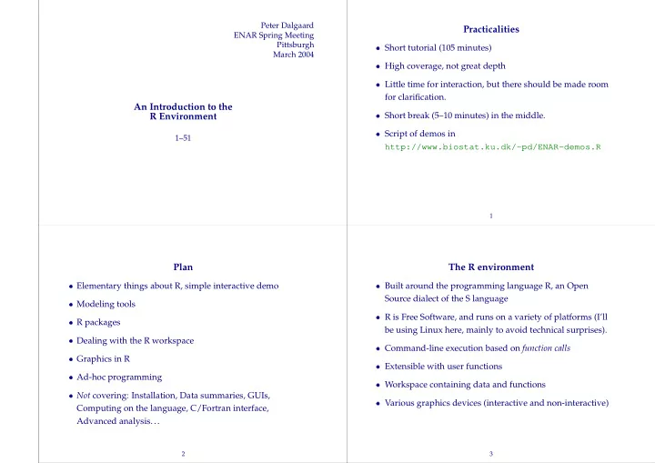
� � � � � � � � � � � � � � � � � � Peter Dalgaard Practicalities ENAR Spring Meeting Pittsburgh Short tutorial (105 minutes) March 2004 High coverage, not great depth Little time for interaction, but there should be made room for clarification. An Introduction to the Short break (5–10 minutes) in the middle. R Environment Script of demos in 1–51 http://www.biostat.ku.dk/~pd/ENAR-demos.R 1 Plan The R environment Elementary things about R, simple interactive demo Built around the programming language R, an Open Source dialect of the S language Modeling tools R is Free Software, and runs on a variety of platforms (I’ll R packages be using Linux here, mainly to avoid technical surprises). Dealing with the R workspace Command-line execution based on function calls Graphics in R Extensible with user functions Ad-hoc programming Workspace containing data and functions Not covering: Installation, Data summaries, GUIs, Various graphics devices (interactive and non-interactive) Computing on the language, C/Fortran interface, Advanced analysis... 2 3
� � � � � � � � � � � � � � � � � The basic vector types Basic operations Standard arithmetic ( x + y , etc.) Numeric (integer/double) Recycling: If operating on two vectors of different length, Character (strings) the shorter one is replicated (with warning if it is not an Logical even multiple) Factor (really integer + level attribute) c — concatenate Lists (generic vectors) seq — sequences rep — replication sum , mean , range , ... 4 5 Demo 1 Smart indexing x <- round(rnorm(10,mean=20,sd=5)) # simulate data a[5] single element x a[5:7] several elements mean(x) a[-6] all except the 6th m <- mean(x) x - m # notice recycling a[b>200] logical index (x - m)^2 a["name"] by name sum((x - m)^2) sqrt(sum((x - m)^2)/9) a$b list elements sd(x) 6 7
� � � � � � � � � � � � � � Matrices/tables/arrays Data frames Used in matrix calculus and as input to, e.g., Like data set in other packages chisq.test() . Results of tabulation. Technically: Lists of vectors/factors of same length Vectors with dimensions Row names (must be unique) Dimnames Indexed like matrices (Beware, though: Data frames are Matrices: Generate with matrix not matrices) Indexing methods include [i,j] , [i,] , [,j] Generate from read operation or with data.frame Many sample data frames are avalilable using data() 8 9 Demo 2 Some standard procedures data(airquality) Continuous data by group: t.test , wilcox.test , airquality$Month oneway.test , kruskal.test airquality[airquality$Month==5,] Categorical data: prop.test , chisq.test , oz <- airquality[airquality$Month==5,]$Ozone fisher.test mean(oz) Correlations: cor.test , with options for nonparametrics mean(oz, na.rm=TRUE) attach(airquality) mean(Ozone, na.rm=TRUE) tapply(Ozone, Month, mean, na.rm=TRUE) detach() 10 11
✂ � ✁ ✁ ✂ � ✁ � ✄ ☎ ✆ � ✁ � ✂ ✄ � � ☎ � ✆ ✁ � � ✁ � � � � � � Demo 3 Modeling tools: Overview library(ISwR) Model formulas data(intake) attach(intake) Model objects and summaries t.test(pre, post, paired=TRUE) Comparing models detach() data(caesarean) # loads a table Evaluating model fit caesar.shoe chisq.test(caesar.shoe) Generalized linear models fisher.test(caesar.shoe) 12 13 Model formulas Model formulas in R R representation y ~ height + type where type is a Linear model, y X β ǫ factor In practice something like Interactions a:b , a*b = a + b + a:b y β 0 β 1 height β 2 1 β 3 1 ǫ type 2 type 3 Algebra ( a:(b + c) = a:b + a:c etc.) Wilkinson-Rogers formulas: Notice special interpretation of operators y height type Special items: offset , -1 (Interpretation depends on whether variables are categorical or continuous) 14 15
� � � � � � � � � � � � � Fitting linear models Inspecting model objects data(airquality) Extract information about the fit aq <- transform(airquality, Month=factor(Month)) fit.aq <- lm(log(Ozone) ~ Solar.R + Wind + summary(fit.aq) Temp + Month, data=aq) fitted , resid lm generates a fitted model object anova(model1, model2) Extract information from model object plot – diagnostics Fit other models based on model object predict(fit.aq, newdata) 16 17 Demo 4 Model search data(airquality) anova(model) “Type I” sum of squares aq <- transform(airquality, Month=factor(Month)) fit.aq <- lm(log(Ozone) ~ Solar.R + Wind + drop1 (“Type III”), add1 Temp + Month, data=aq) step (AIC/BIC) criteria fit.aq2 <- update(fit.aq, ~ . - Month) summary(fit.aq) update plot(fit.aq) drop1(fit.aq, test="F") anova(fit.aq, fit.aq2) 18 19
✁ � � � � ✁ � � ✂ � � � � ☎ � � ✂ � ✄ � � � Demo 5 Generalized linear models no.yes <- c("No","Yes") Statistical distribution (exponential) family smoking <- gl(2, 1, 8, no.yes) obesity <- gl(2, 2, 8, no.yes) Link function transforming mean to linear scale snoring <- gl(2, 4, 8, no.yes) Deviance n.tot <- c(60,17,8,2,187,85,51,23) n.hyp <- c(5,2,1,0,35,13,15,8) Examples; Binomial, Poisson, Gaussian ( σ known — in data.frame(smoking,obesity,snoring,n.tot,n.hyp) principle) hyp.tbl <- cbind(n.hyp,n.tot-n.hyp) glm.hyp <- glm(hyp.tbl~smoking+obesity+snoring, Canonical link functions family=binomial("logit")) summary(glm.hyp) Fit using glm in R 0.87194 + qnorm(c(.025,.975))*0.39757 library(MASS) confint(glm.hyp) 20 21 Likelihood-based inference R packages Wald approximations ( ˆ ˆ s.e. , etc.) can be badly β β Collections of R functions, data, and compiled code inaccurate in small samples Well-defined format that ensures easy installation, a basic Likelihood-based inference is preferable standard of documentation, and enhances portability and reliability, Use drop1(model, test="Chisq") (for binomial/Poisson) You can write your own packages! It is not entirely trivial, but tools are there to help you. profile (in MASS for glm ) investigates behaviour of likelihood around maximum plot(profile(model)) shows signed LR statistic ˆ sign β β Q when varying each parameter. confint gives likelihood-based confidence intervals 22 23
� � � � � � � � � � � � � Packages that come with R CRAN The Comprehensive R Archive Network Standard R (1.8.1 - reorganized in 1.9.0) loads with these packages available Collection of servers mirroring a central server in Vienna. – ctest — Classical tests Modeled on CTAN and CPAN (for TEX and Perl code) – mva — Multivariate analysis http://cran.us.r-project.org – modreg — Modern Regression Maintains a curated collection of R packages as well as the – nls — Nonlinear regression source and binary distributions R itself – ts — Time series (elementary) About 320 packages available 8 further packages are available in core R, but not Unix/Linux variants generally install packages from automatically loaded ( tcltk , lqs , ...) sources. Windows and MacOSX have binary package formats which are even easier to install 10 further packages and package bundles are maintained separately, but included with source and binary See also: Bioconductor, http://www.bioconductor.org distributions ( survival , nlme , MASS , ...). 24 25 Demo 6 Practical issues # Cheat for offline demo: Dealing with the workspace # Pretend CRAN is local directory options(CRAN="file:/home/pd/cran.r-project.org") Reading data # Manipulate install path Saving and restoring data and results .libPaths("~/Rlibrary") .libPaths() # Source install (gives harmless warning) install.packages("mvtnorm") library(mvtnorm) library(help=mvtnorm) 26 27
� � � � � � � � � � � � � � Demo 7 The workspace search() The global environment contains R objects created on the data(intake) # From ISwR command line. ls() attach(intake) There is an additional search path of loaded packages and search() attached data frames. ls("intake") # show variables in data frame post - pre The search path is maintained by library() , attach() , rm(intake) # remove data frame and detach() detach() # remove from search path This determines the way R looks up objects by name Notice that objects in the global environment may mask objects in packages. 28 29 Reading data Getting organized Simple data vectors can be read using scan() Several possibilities: Data frames can be read from most reasonably structured Save/restore entire workspace (objects only) text file formats (space separated columns, tab- and Save selected objects and load them comma-delimited files) using read.table() or source() script files read.delim() . Batch processing ( R CMD BATCH file.R ) The read functions have many useful arguments. Notice in particular colClasses , which allows you setup ad-hoc ESS – Emacs Speaks Statistics: Integrated environment for conversion to any desired object class. maintaining scripts, running R, saving results, etc. The foreign package can read files from Stata, SAS export libraries, SPSS, and Epi-Info, Minitab, and some S-PLUS versions. 30 31
Recommend
More recommend
Explore More Topics
Stay informed with curated content and fresh updates.

