Polynomial Invariant Generation for Non-deterministic Recursive - PowerPoint PPT Presentation
Polynomial Invariant Generation for Non-deterministic Recursive Programs Krishnendu Chatterjee 1 , Hongfei Fu 2 Amir Kafshdar Goharshady 1 , Ehsan Kafshdar Goharshady 3 1 IST Austria 2 Shanghai Jiao Tong University 3 Ferdowsi University of Mashhad
Polynomial Invariant Generation for Non-deterministic Recursive Programs Krishnendu Chatterjee 1 , Hongfei Fu 2 Amir Kafshdar Goharshady 1 , Ehsan Kafshdar Goharshady 3 1 IST Austria 2 Shanghai Jiao Tong University 3 Ferdowsi University of Mashhad
Invariants ◮ An assertion at a point of the program that holds whenever a valid execution reaches that point ◮ An over-approximation of the set of reachable states
Inductive Invariants Let C be a set of program locations that is visited by every cycle. An Inductive Invariant is an assertion A l at every location l ∈ C , such that for each l , l ′ ∈ C : ◮ Initiation: A l holds in the first visit to l . ◮ Consecution: If A l holds at l , then every simple path from l to l ′ ensures that A l ′ holds at l ′ . In the sequel, we assume C = L , i.e. every label is in C . The primary method to show that an assertion is an invariant is to generate an inductive invariant that strengthens it.
Previous Works on Invariant Generation
Polynomial Invariants ◮ Consider programs with polynomial guards/assignments ◮ Goal: Generate invariants that are conjunctions of polynomial inequalities Pick Two: ◮ Automation ◮ Completeness ◮ Applicability Placeholder Placeholder
Polynomial Invariants Pick Two: ◮ Automation ◮ Completeness ◮ Applicability “Automatically Generating Loop Invariants using Quantifier Elimination” (Kapur, ACA 2004)
Polynomial Invariants Pick Two: ◮ Automation ◮ Completeness ◮ Applicability “Non-linear Reasoning for Invariant Synthesis” (Kincaid, Cyphert, Breck, and Reps, POPL 2018)
Polynomial Invariants Pick Two: ◮ Automation ◮ Completeness ◮ Applicability Interactive Theorem Provers Not the subject of this talk!
Why not all three?
A Simple Example Precondition: 100 − y 2 ≥ 0 x 2 − 100 ≥ 0 then i f Invariant: c 1 · y 2 + c 2 · y + c 3 ≥ 0 x := y else Invariant: c 4 · x 2 + c 5 · x + c 6 ≥ 0 skip f i Postcondition: c 7 · x + c 8 ≥ 0 ◮ 100 − y 2 ≥ 0 ∧ x 2 − 100 ≥ 0 ⇒ c 1 · y 2 + c 2 · y + c 3 ≥ 0 ◮ 100 − y 2 ≥ 0 ∧ 100 − x 2 > 0 ⇒ c 4 · x 2 + c 5 · x + c 6 ≥ 0 ◮ c 1 · y 2 + c 2 · y + c 3 ≥ 0 ⇒ c 7 · y + c 8 ≥ 0 ◮ c 4 · x 2 + c 5 · x + c 6 ≥ 0 ⇒ c 7 · x + c 8 ≥ 0
A Simple Example Precondition: 100 − y 2 ≥ 0 x 2 − 100 ≥ 0 then i f Invariant: − 1 · y 2 + 0 · y + 100 ≥ 0 x := y else Invariant: c 4 · x 2 + c 5 · x + c 6 ≥ 0 skip f i Postcondition: c 7 · x + c 8 ≥ 0 ◮ 100 − y 2 ≥ 0 ∧ x 2 − 100 ≥ 0 ⇒ − 1 · y 2 + 0 · y + 100 ≥ 0 ◮ 100 − y 2 ≥ 0 ∧ 100 − x 2 > 0 ⇒ c 4 · x 2 + c 5 · x + c 6 ≥ 0 ◮ − 1 · y 2 + 0 · y + 100 ≥ 0 ⇒ c 7 · y + c 8 ≥ 0 ◮ c 4 · x 2 + c 5 · x + c 6 ≥ 0 ⇒ c 7 · x + c 8 ≥ 0
A Simple Example Precondition: 100 − y 2 ≥ 0 x 2 − 100 ≥ 0 then i f Invariant: − 1 · y 2 + 0 · y + 100 ≥ 0 x := y else Invariant: − 1 · x 2 + 0 · x + 100 ≥ 0 skip f i Postcondition: c 7 · x + c 8 ≥ 0 ◮ 100 − y 2 ≥ 0 ∧ x 2 − 100 ≥ 0 ⇒ − 1 · y 2 + 0 · y + 100 ≥ 0 ◮ 100 − y 2 ≥ 0 ∧ 100 − x 2 > 0 ⇒ − 1 · x 2 + 0 · x + 100 ≥ 0 ◮ − 1 · y 2 + 0 · y + 100 ≥ 0 ⇒ c 7 · y + c 8 ≥ 0 ◮ − 1 · x 2 + 0 · x + 100 ≥ 0 ⇒ c 7 · x + c 8 ≥ 0
A Simple Example ◮ 100 − y 2 ≥ 0 ⇒ c 7 · y + c 8 ≥ 0 ◮ ( a · y − b ) 2 ≥ 0 ∧ 100 − y 2 ≥ 0 ⇒ c 7 · y + c 8 ≥ 0 ◮ c 7 · y + c 8 = ( a · y − b ) 2 + d · (100 − y 2 ) ◮ c 7 · y + c 8 = a 2 · y 2 − 2 · a · b · y + b 2 + 100 · d − d · y 2 ◮ 0 = a 2 − d ◮ c 7 = − 2 · a · b ◮ c 8 = b 2 + 100 · d √ 1 1 ◮ One solution: a = 5 , b = 5 , d = 20 , c 7 = − 1 , c 8 = 10 √ 2 ◮ In other words � 1 � 2 √ + 1 20(100 − y 2 ) 10 − y = √ · y − 5 2 5 So we can safely deduce: 100 − y 2 ≥ 0 ⇒ 10 − y ≥ 0
A Simple Example Precondition: 100 − y 2 ≥ 0 x 2 − 100 ≥ 0 then i f Invariant: − 1 · y 2 + 0 · y + 100 ≥ 0 x := y else Invariant: − 1 · x 2 + 0 · x + 100 ≥ 0 skip f i Postcondition: − 1 · x + 10 ≥ 0 ◮ 100 − y 2 ≥ 0 ∧ x 2 − 100 ≥ 0 ⇒ − 1 · y 2 + 0 · y + 100 ≥ 0 ◮ 100 − y 2 ≥ 0 ∧ 100 − x 2 > 0 ⇒ − 1 · x 2 + 0 · x + 100 ≥ 0 ◮ − 1 · y 2 + 0 · y + 100 ≥ 0 ⇒ − 1 · y + 10 ≥ 0 ◮ − 1 · x 2 + 0 · x + 100 ≥ 0 ⇒ − 1 · x + 10 ≥ 0
Outline 1. Generate a Template ◮ For example, A 1 := c 0 + c 1 · x + c 2 · y + c 3 · x 2 + c 4 · x · y + c 5 · y 2 ≥ 0 2. Compute Inductivity Conditions (Initiation and Consecution) ◮ Each such condition is of this form: g 1 ≥ 0 ∧ g 2 ≥ 0 ∧ . . . ∧ g m ≥ 0 ⇒ g ≥ 0 3. Handle the condition by writing g as a combination of g i ’s: m � g = h 0 + h i · g i (1) i =1 where the h i ’s are polynomials whose coefficients are new unknowns. ◮ For example, h 0 = a 0 + a 1 · x + a 2 · y + a 3 · x 2 + a 4 · x · y + a 5 · y 2 4. Equate corresponding coefficients on the two sides of (1). 5. Add extra conditions on the coefficients of h i ’s, ensuring that they are SOS. 6. Solve the resulting quadratic system.
Soundness Soundness is trivial. Assuming every g i is non-negative, and given that every h i is a SOS, we can directly infer that m � g = h 0 + g i · h i i =1 is also non-negative.
Completeness Theorem (Putinar’s Positivstellensatz) Let V be a finite set of variables and g , g 1 , . . . , g m ∈ R [ V ] polynomials over V with real coefficients. We define Π := { x ∈ R V | ∀ i g i ( x ) ≥ 0 } as the set of points in which every g i is non-negative. If (i) there exists some g k s.t. the set { x ∈ R V | g k ( x ) ≥ 0 } is compact, and (ii) g ( x ) > 0 for all x ∈ Π , then m � g = h 0 + h i · g i i =1 where each polynomial h i is SOS. Theorem (See details in the paper) Under certain conditions, our approach is complete for invariants that are a conjunction of strict polynomial inequalities.
Complexity and Applicability If we fix the degree of all polynomials and the length of invariant at every point of the program, then our approach is a polynomial-time reduction from Invariant Generation to QP.
Experimental Results Times are reported in seconds. Time limit was 12 hours per instance. Humenberger et al, Benchmark Ours ICRA SeaHorn UAutomizer Kapur, ACA 2004 ISSAC 2017 cohendiv 15.2 0.7 0.1 3.3 Not Applicable Timed Out divbin 5.4 Failed Timed Out 0.2 Failed Timed Out hard 28.0 Failed Failed 0.4 Failed Timed Out mannadiv 18.2 Failed 0.1 0.1 Timed Out Timed Out wensely 20.1 0.1 Failed Failed Failed Timed Out sqrt 5.8 0.8 0.1 Failed Timed Out Timed Out dijkstra 12.8 Failed Failed Not Applicable Failed Timed Out z3sqrt 12.9 0.5 0.1 Not Applicable Failed Timed Out freire1 26.5 0.6 Failed 0.1 Failed Timed Out freire2 10.7 1.1 0.1 Failed Failed Timed Out euclidex1 97.5 Failed Failed Not Applicable Timed Out Timed Out euclidex2 39.3 0.4 Failed Failed Timed Out Timed Out euclidex3 203.1 Failed Failed Not Applicable Timed Out Timed Out lcm1 17.9 0.8 0.1 Not Applicable 3.7 Timed Out lcm2 18.7 0.8 0.1 0.1 3.2 Timed Out prodbin 12.1 Failed Failed Not Applicable Timed Out Timed Out prod4br 43.2 Failed Failed Not Applicable Timed Out Timed Out cohencu 11.8 0.6 0.1 Failed Timed Out Timed Out petter 20.4 0.5 0.1 0.1 2.7 Timed Out
Summary For Polynomial Invariant Generation, we can have all three: ◮ Automation: Push-button approach ◮ Completeness: Through Putinar’s Positivstellensatz ◮ Applicability: Reduction to QP See the paper for proofs and extension to recursive programs! The research was partially supported by Austrian Science Fund (FWF) Grant No. NFN S11407-N23 (RiSE/SHiNE), Vienna Science and Technology Fund (WWTF) Project ICT15-003, National Natural Science foundation of China (NSFC) Grant No. 61802254, the Facebook PhD Fellowship Program, and DOC Fellowship No. 24956 of the Austrian Academy of Sciences (¨ OAW).
Recommend
More recommend
Explore More Topics
Stay informed with curated content and fresh updates.


