Phase Noise Enrico Rubiola Dept. LPMO, FEMTO ST Institute - PowerPoint PPT Presentation

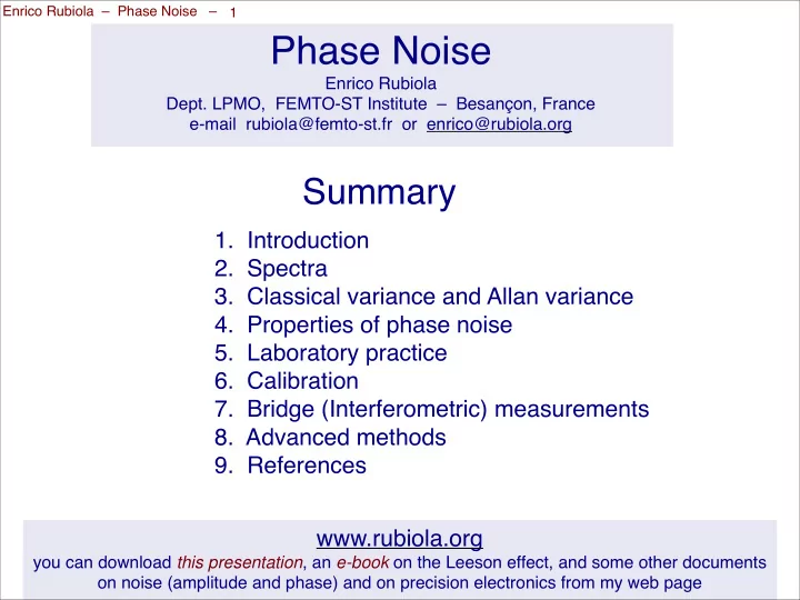
Enrico Rubiola – Phase Noise – 1 Phase Noise Enrico Rubiola Dept. LPMO, FEMTO ­ ST Institute – Besançon, France e ­ mail rubiola@femto ­ st.fr or enrico@rubiola.org Summary 1. Introduction 2. Spectra 3. Classical variance and Allan variance 4. Properties of phase noise 5. Laboratory practice 6. Calibration 7. Bridge (Interferometric) measurements 8. Advanced methods 9. References www.rubiola.org you can download this presentation , an e-book on the Leeson effect, and some other documents on noise (amplitude and phase) and on precision electronics from my web page

Enrico Rubiola – Phase Noise – 2 1 – Introduction

introduction – noisy sinusoid Enrico Rubiola – Phase Noise – 3 Representations of a sinusoid with noise Time Domain Phasor Representation amplitude fluctuation v ( t ) V 0 α ( t ) [volts] V 0 normalized ampl. fluct. α ( t ) [adimensional] √ V 0 / 2 t ampl. fluct. √ ( V 0 / 2) α ( t ) phase fluctuation v ( t ) ϕ ( t ) [rad] V 0 phase fluctuation phase time (fluct.) x ( t ) [seconds] ϕ ( t ) t √ V 0 / 2 v ( t ) = V 0 [1 + α ( t )] cos [ ω 0 t + ϕ ( t )] polar coordinates v ( t ) = V 0 cos ω 0 t + n c ( t ) cos ω 0 t − n s ( t ) sin ω 0 t Cartesian coordinates under low noise approximation It holds that α ( t ) = n c ( t ) ϕ ( t ) = n s ( t ) and | n c ( t ) | ≪ V 0 and | n s ( t ) | ≪ V 0 V 0 V 0

introduction – noisy sinusoid Enrico Rubiola – Phase Noise – 4 Noise broadens the spectrum v ( t ) = V 0 [1 + α ( t )] cos [ ω 0 t + ϕ ( t )] v ( t ) = V 0 cos ω 0 t + n c ( t ) cos ω 0 t − n s ( t ) sin ω 0 t ω = 2 πν ν = ω 2 π

introduction – general problems Enrico Rubiola – Phase Noise – 5 Basic problem: how can we measure a low random signal (noise sidebands) close to a strong dazzling carrier? solution(s): suppress the carrier and measure the noise convolution distorsiometer, s ( t ) ∗ h lp ( t ) audio-frequency instruments (low-pass) traditional instruments for time-domain s ( t ) × r ( t − T/ 4) phase-noise measurement product (saturated mixer) vector bridge (interferometric) s ( t ) − r ( t ) instruments difference

introduction – general problems Enrico Rubiola – Phase Noise – 6 Why a spectrum analyzer does not work? 1. too wide IF bandwidth 2. noise and instability of the conversion oscillator (VCO) 3. detects both AM and PM noise 4. insufficient dynamic range Some commercial analyzers provide phase noise measurements, yet limited (at least) by the oscillator stability

introduction – φ –> v converter Enrico Rubiola – Phase Noise – 7 The Schottky-diode double-balanced mixer saturated at both inputs is the most used phase detector � signal s ( t ) = 2 R 0 P 0 cos [2 πν 0 t + ϕ ( t )] � r ( t ) = 2 R 0 P 0 cos [2 πν 0 t + π / 2] reference filtered out r ( t ) s ( t ) = k ϕ ϕ ( t ) + “2 ν 0 ” terms product The AM noise is rejected by saturation Saturation also account for the phase-to-voltage gain k φ

Enrico Rubiola – Phase Noise – 8 2 – Spectra

Spectra – definitions Enrico Rubiola – Phase Noise – 9 Power spectrum density In general, the power spectrum density S v (f) of a random process v(t) is defined as � �� � S v ( f ) = E R v ( t 1 , t 2 ) F � � E statistical expectation · � � F · Fourier transform R v ( t 1 , t 2 ) autocorrelation function In practice, we measure S v (f) as � 2 � �� � S v ( f ) = v ( t ) � F This is possible (Wiener-Khinchin theorem) with ergodic processes In many real-life cases, processes are ergodic and stationary Ergodicity: ensemble and time-domain statistics can be interchanged. This is the formalization of the reproducibility of an experiment Stationarity: the statistics is independent of the origin of time. This is the formalization of the repeatability of an experiment

Spectra – meaning Enrico Rubiola – Phase Noise – 10 Physical meaning of the power spectrum density P = S v ( f 0 ) R 0 S v ( f 0 ) power in 1 Hz bandwidth dissipated by R 0 R 0

Spectra – meaning Enrico Rubiola – Phase Noise – 11 Physical meaning of the power spectrum density The power spectrum density extends the concept of root-mean-square value to the frequency domain

Spectra – S φ (f) and ℒ (f) Enrico Rubiola – Phase Noise – 12 S φ (f) and ℒ (f) in the presence of (white) noise SSB DSB P 0 P 0 B B B N N v 0 v 0 v v 0 – v 0 v 0 v +f f +f ϕ p ϕ p � � R 0 NB/ 2 R 0 NB � � R 0 P 0 R 0 P 0 � � � � NB NB 1 1 ϕ rms = 2 ϕ p = ϕ rms = 2 ϕ p = 2 P 0 P 0 S ϕ = N L = N 3 dB dBc/Hz dBrad 2 /Hz P 0 2 P 0

Spectra – S φ (f) and ℒ (f) Enrico Rubiola – Phase Noise – 13 ℒ (f) (re)defined The first definition of ℒ (f) was ℒ (f) = ( SSB power in 1Hz bandwidth ) / ( carrier power ) The problem with this definition is that it does not divide AM noise from PM noise, which yields to ambiguous results Engineers (manufacturers even more) like ℒ (f) The IEEE Std 1139-1999 redefines ℒ (f) as ℒ (f) = (1/2) × S φ (f)

Spectra – useful quantities Enrico Rubiola – Phase Noise – 14 Useful quantities 1 phase x ( t ) = ϕ ( t ) time 2 πν 0 x(t) is the phase noise converted into time fluctuation physical dimension: time (seconds) fractional 1 y ( t ) = ϕ ( t ) = ˙ ˙ x ( t ) frequency 2 πν 0 fluctuation y(t) is the fractional frequency fluctuation ν - ν 0 normalized to the nominal frequency ν 0 y ( t ) = ν − ν 0 (dimensionless) ν 0

Spectra – power law Enrico Rubiola – Phase Noise – 15 Power-law and noise processes in oscillators

Spectra – power law Enrico Rubiola – Phase Noise – 16 Relationships between S φ (f) and S y (f)

Spectra – jitter Enrico Rubiola – Phase Noise – 17 Jitter The phase fluctuation can be described in terms of a single parameter, either phase jitter or time jitter The phase noise must be integrated over the bandwidth B of the system (which may be difficult to identify) & rms ! $ % S & ' f ( df radians phase jitter B 2 "# 0 $ % 1 time jitter S & ' f ( df x rms ! seconds phase jitter B converted into time The jitter is useful in digital circuits because the bandwidth B is known – lower limit: the inverse propagation time through the system this excludes the low-frequency divergent processes) – upper limit: ~ the inverse switching speed Victor Reinhardt (invited), A Review of Time Jitter and Digital Systems, Proc. 2005 FCS-PTTI joint meeting

Spectra – examples Enrico Rubiola – Phase Noise – 18 Typical phase noise of some devices and oscillators 1 0 G 1 H 0 -40 z G D H i e z l e S c a t r p i p c -60 h R i r e e 1 s o 0 R n G e a s t H o o n z r -80 a O S t o R s S (f) (dBrad /Hz) 100 MHz quartz oscillator r c O i O l l w s a c t i o i t l h r l a n -100 t o o 2 i r s ( e S d R e O g e ) n -120 e microwave amplifier r a t i o n RF amplifier 5 MHz quartz osc. -140 � -160 microwave ferrite isolators -180 -200 -200 -200 0.1 1 10 100 1k 10k 100k Fourier frequency (Hz)

Enrico Rubiola – Phase Noise – 19 3 – Variances

Variances – classical Enrico Rubiola – Phase Noise – 20 Classical variance 1 1 # $ normalized reading of a counter that y ! "% t & dt " 0 measures (averages) over a time T # % y i ( 1 y j & 2 N N ' 2 ! 1 classical variance, N ( 1 ) N ) file of N counter readings i ! 1 j ! 1 average of the N readings For a given process, the classical variance depends of N Even worse, if the spectrum is f -1 or steeper, the classical variance diverges The filter associated to the measure takes in the dc component

Variances – Allan Enrico Rubiola – Phase Noise – 21 Zero dead-time two-sample variance (Allan variance) 2 # $ y 2 % y 1 & 2 ' 2 " 1 Definition ! y (Let N = 2, and average) m % 1 Estimated Allan variance, 2 " 1 2 $ m % 1 & ( $ y 2 % y 1 & 2 ! y file of m counter readings i " 1 The filter associated to the difference of two contiguous measures is a band-pass The estimate converges to the variance

Variances – Allan Enrico Rubiola – Phase Noise – 22 The Allan variance is related to the spectrum S y (f)

Variances – Allan Enrico Rubiola – Phase Noise – 23 Convert S φ and S y into Allan variance noise σ 2 mod σ 2 S ϕ ( f ) S y ( f ) y ( τ ) y ( τ ) S ϕ ↔ S y type 3 f H h 2 (2 π ) 2 τ − 2 3 f H τ 0 h 2 white h 2 = b 0 τ − 3 h 2 f 2 b 0 PM ν 2 (2 π ) 2 0 2 πτ f H ≫ 1 h 1 0 . 084 h 1 τ − 2 flicker h 1 = b − 1 (2 π ) 2 τ − 2 b − 1 f − 1 [1 . 038+3 ln(2 π f H τ )] h 1 f PM ν 2 n ≫ 1 0 1 1 white h 0 = b − 2 2 h 0 τ − 1 4 h 0 τ − 1 b − 2 f − 2 h 0 FM ν 2 0 27 flicker h − 1 = b − 3 h − 1 f − 1 b − 3 f − 3 2 ln(2) h − 1 20 ln(2) h − 1 FM ν 2 0 random (2 π ) 2 0 . 824 (2 π ) 2 h − 2 = b − 4 b − 4 f − 4 h − 2 f − 2 walk h − 2 τ h − 2 τ ν 2 6 6 FM 0 1 1 2 D 2 y τ 2 2 D 2 y τ 2 frequency drift ˙ y = D y f H is the high cuto ff frequency, needed for the noise power to be finite.

Enrico Rubiola – Phase Noise – 24 4 – Properties of phase noise