Personalized screening intervals for biomarkers using joint models - PowerPoint PPT Presentation

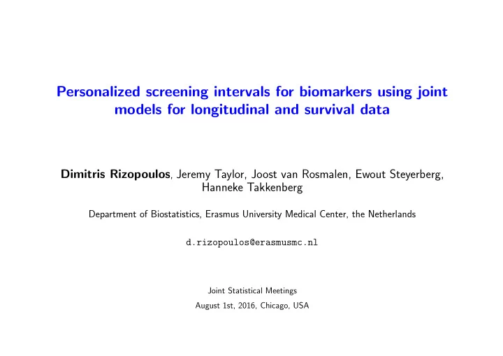
Personalized screening intervals for biomarkers using joint models for longitudinal and survival data Dimitris Rizopoulos , Jeremy Taylor, Joost van Rosmalen, Ewout Steyerberg, Hanneke Takkenberg Department of Biostatistics, Erasmus University Medical Center, the Netherlands d.rizopoulos@erasmusmc.nl Joint Statistical Meetings August 1st, 2016, Chicago, USA

1. Introduction • Nowadays growing interest in tailoring medical decision making to individual patients ◃ Personalized Medicine ◃ Shared Decision Making • This is of high relevance in various diseases ◃ cancer research, cardiovascular diseases, HIV research, . . . Physicians are interested in accurate prognostic tools that will inform them about the future prospect of a patient in order to adjust medical care JSM – August 1st, 2016, Chicago 1/30

1. Introduction (cont’d) • Aortic Valve study: Patients who received a human tissue valve in the aortic position ◃ data collected by Erasmus MC (from 1987 to 2008); 77 received sub-coronary implantation; 209 received root replacement • Outcomes of interest: ◃ death and re-operation → composite event ◃ aortic gradient JSM – August 1st, 2016, Chicago 2/30

1. Introduction (cont’d) • General Questions: ◃ Can we utilize available aortic gradient measurements to predict survival/re-operation? ◃ When to plan the next echo for a patient? JSM – August 1st, 2016, Chicago 3/30

1. Introduction (cont’d) • Goals of this talk : ◃ introduce joint models ◃ dynamic predictions ◃ optimal timing of next visit JSM – August 1st, 2016, Chicago 4/30

2.1 Joint Modeling Framework • To answer these questions we need to postulate a model that relates ◃ the aortic gradient with ◃ the time to death or re-operation • Some notation ◃ T ∗ i : True time-to-death for patient i ◃ T i : Observed time-to-death for patient i ◃ δ i : Event indicator, i.e., equals 1 for true events ◃ y i : Longitudinal aortic gradient measurements JSM – August 1st, 2016, Chicago 5/30

2.1 Joint Modeling Framework (cont’d) hazard 0.4 0.3 0.2 0.1 marker 2.0 1.5 1.0 0.5 0.0 0 2 4 6 8 Time JSM – August 1st, 2016, Chicago 6/30

2.1 Joint Modeling Framework (cont’d) • We start with a standard joint model ◃ Survival Part: Relative risk model h i ( t | M i ( t )) = h 0 ( t ) exp { γ ⊤ w i + αm i ( t ) } , where * m i ( t ) = the true & unobserved value of aortic gradient at time t * M i ( t ) = { m i ( s ) , 0 ≤ s < t } * α quantifies the effect of aortic gradient on the risk for death/re-operation * w i baseline covariates JSM – August 1st, 2016, Chicago 7/30

2.1 Joint Modeling Framework (cont’d) ◃ Longitudinal Part: Reconstruct M i ( t ) = { m i ( s ) , 0 ≤ s < t } using y i ( t ) and a mixed effects model (we focus on continuous markers) y i ( t ) = m i ( t ) + ε i ( t ) = x ⊤ i ( t ) β + z ⊤ ε i ( t ) ∼ N (0 , σ 2 ) , i ( t ) b i + ε i ( t ) , where * x i ( t ) and β : Fixed-effects part * z i ( t ) and b i : Random-effects part, b i ∼ N (0 , D ) JSM – August 1st, 2016, Chicago 8/30

2.1 Joint Modeling Framework (cont’d) • The two processes are associated ⇒ define a model for their joint distribution • Joint Models for such joint distributions are of the following form (Tsiatis & Davidian, Stat. Sinica , 2004; Rizopoulos, CRC Press, 2012) ∫ { } h ( T i | b i ) δ i S ( T i | b i ) p ( y i | b i ) p ( y i , T i , δ i ) = p ( b i ) db i where ◃ b i a vector of random effects that explains the interdependencies ◃ p ( · ) density function; S ( · ) survival function JSM – August 1st, 2016, Chicago 9/30

2.2 Estimation • Joint models can be estimated with either Maximum Likelihood or Bayesian approaches (i.e., MCMC) • Here we follow the Bayesian approach because it facilitates computations for our later developments. . . JSM – August 1st, 2016, Chicago 10/30

3.1 Prediction Survival – Definitions • We are interested in predicting survival probabilities for a new patient j that has provided a set of aortic gradient measurements up to a specific time point t • Example: We consider Patients 20 and 81 from the Aortic Valve dataset JSM – August 1st, 2016, Chicago 11/30

3.1 Prediction Survival – Definitions (cont’d) 0 5 10 Patient 20 Patient 81 10 8 Aortic Gradient (mmHg) 6 4 2 0 0 5 10 Follow−up Time (years) JSM – August 1st, 2016, Chicago 12/30

3.1 Prediction Survival – Definitions (cont’d) 2 4 6 8 10 12 Patient 20 Patient 81 10 Aortic Gradient (mmHg) 8 6 4 2 0 2 4 6 8 10 12 Follow−up Time (years) JSM – August 1st, 2016, Chicago 12/30

3.1 Prediction Survival – Definitions (cont’d) 2 4 6 8 10 12 Patient 20 Patient 81 10 Aortic Gradient (mmHg) 8 6 4 2 0 2 4 6 8 10 12 Follow−up Time (years) JSM – August 1st, 2016, Chicago 12/30

3.1 Prediction Survival – Definitions (cont’d) • What do we know for these patients? ◃ a series of aortic gradient measurements ◃ patient are event-free up to the last measurement • Dynamic Prediction survival probabilities are dynamically updated as additional longitudinal information is recorded JSM – August 1st, 2016, Chicago 13/30

3.1 Prediction Survival – Definitions (cont’d) • Available info: A new subject j with longitudinal measurements up to t ◃ T ∗ j > t ◃ Y j ( t ) = { y j ( t jl ); 0 ≤ t jl ≤ t, l = 1 , . . . , n j } ◃ D n sample on which the joint model was fitted Basic tool: Posterior Predictive Distribution { } T ∗ j | T ∗ j > t, Y j ( t ) , D n p JSM – August 1st, 2016, Chicago 14/30

3.2 Prediction Survival – Estimation • Based on the fitted model we can estimate the conditional survival probabilities { } T ∗ j ≥ u | T ∗ π j ( u | t ) = Pr j > t, Y j ( t ) , D n , u > t • For more details check: ◃ Proust-Lima and Taylor (2009, Biostatistics), Rizopoulos (2011, Biometrics), Taylor et al. (2013, Biometrics) JSM – August 1st, 2016, Chicago 15/30

3.3 Prediction Survival – Illustration • Example: We fit a joint model to the Aortic Valve data • Longitudinal submodel ◃ fixed effects: natural cubic splines of time (d.f. = 3 ), operation type, and their interaction ◃ random effects: Intercept, & natural cubic splines of time (d.f. = 3 ) • Survival submodel ◃ type of operation, age, sex + underlying aortic gradient level ◃ log baseline hazard approximated using B-splines JSM – August 1st, 2016, Chicago 16/30

3.3 Prediction Survival – Illustration (cont’d) 0 5 10 Patient 20 Patient 81 10 8 Aortic Gradient (mmHg) 6 4 2 0 0 5 10 Follow−up Time (years) JSM – August 1st, 2016, Chicago 17/30

3.3 Prediction Survival – Illustration (cont’d) Patient 81 Patient 20 1.0 1.0 12 12 10 10 0.8 0.8 Re−Operation−Free Survival Aortic Gradient (mmHg) 8 8 0.6 0.6 6 6 0.4 0.4 4 4 0.2 0.2 2 2 0 0 0.0 0.0 0 5 10 15 0 5 10 15 Time Time JSM – August 1st, 2016, Chicago 18/30

3.3 Prediction Survival – Illustration (cont’d) Patient 81 Patient 20 1.0 1.0 12 12 10 10 0.8 0.8 Re−Operation−Free Survival Aortic Gradient (mmHg) 8 8 0.6 0.6 6 6 0.4 0.4 4 4 0.2 0.2 2 2 0 0 0.0 0.0 0 5 10 15 0 5 10 15 Time Time JSM – August 1st, 2016, Chicago 18/30

3.3 Prediction Survival – Illustration (cont’d) Patient 81 Patient 20 1.0 1.0 12 12 10 10 0.8 0.8 Re−Operation−Free Survival Aortic Gradient (mmHg) 8 8 0.6 0.6 6 6 0.4 0.4 4 4 0.2 0.2 2 2 0 0 0.0 0.0 0 5 10 15 0 5 10 15 Time Time JSM – August 1st, 2016, Chicago 18/30

3.3 Prediction Survival – Illustration (cont’d) Patient 81 Patient 20 1.0 1.0 12 12 10 10 0.8 0.8 Re−Operation−Free Survival Aortic Gradient (mmHg) 8 8 0.6 0.6 6 6 0.4 0.4 4 4 0.2 0.2 2 2 0 0 0.0 0.0 0 5 10 15 0 5 10 15 Time Time JSM – August 1st, 2016, Chicago 18/30

3.3 Prediction Survival – Illustration (cont’d) Patient 81 Patient 20 1.0 1.0 12 12 10 10 0.8 0.8 Re−Operation−Free Survival Aortic Gradient (mmHg) 8 8 0.6 0.6 6 6 0.4 0.4 4 4 0.2 0.2 2 2 0 0 0.0 0.0 0 5 10 15 0 5 10 15 Time Time JSM – August 1st, 2016, Chicago 18/30

3.3 Prediction Survival – Illustration (cont’d) Patient 81 Patient 20 1.0 1.0 12 12 10 10 0.8 0.8 Re−Operation−Free Survival Aortic Gradient (mmHg) 8 8 0.6 0.6 6 6 0.4 0.4 4 4 0.2 0.2 2 2 0 0 0.0 0.0 0 5 10 15 0 5 10 15 Time Time JSM – August 1st, 2016, Chicago 18/30

4.1 Next Visit Time – Set up • Question 2: ◃ When the patient should come for the next visit? JSM – August 1st, 2016, Chicago 19/30

4.1 Next Visit Time – Set up (cont’d) This is a difficult question! • Many parameters that affect it ◃ which model to use? ◃ what criterion to use? ◃ change in treatment? ◃ . . . We will work under the following setting ⇒ JSM – August 1st, 2016, Chicago 20/30

4.1 Next Visit Time – Set up(cont’d) Event−Free Probability AoGradient t Time JSM – August 1st, 2016, Chicago 21/30

4.1 Next Visit Time – Set up(cont’d) Event−Free Probability AoGradient t Time JSM – August 1st, 2016, Chicago 21/30

4.1 Next Visit Time – Set up(cont’d) Event−Free Probability AoGradient t u Time JSM – August 1st, 2016, Chicago 21/30