Permanents and the Jones polynomial Iain Moffatt 1 Martin Loebl 2 1 - PowerPoint PPT Presentation
Permanents and the Jones polynomial Iain Moffatt 1 Martin Loebl 2 1 University of South Alabama 2 Charles University Summer Combo in Vermont, 13 th July 2012 Permanents Determinant of an n n matrix A = [ a ij ] n det ( A ) := sgn (
Permanents and the Jones polynomial Iain Moffatt 1 Martin Loebl 2 1 University of South Alabama 2 Charles University Summer Combo in Vermont, 13 th July 2012
Permanents Determinant of an n × n matrix A = [ a ij ] n � � det ( A ) := sgn ( σ ) a i σ ( i ) σ ∈ S n i = 1 a b c = aei − afh + dch − dbi + gbf − gce det d e f g h i Permanent of an n × n matrix A = [ a ij ] n � � per ( A ) := a i σ ( i ) σ ∈ S n i = 1 a b c = aei + afh + dch + dbi + gbf + gce per d e f g h i
Permanents Determinant of an n × n matrix A = [ a ij ] n � � det ( A ) := sgn ( σ ) a i σ ( i ) σ ∈ S n i = 1 a b c = aei − afh + dch − dbi + gbf − gce det d e f g h i Permanent of an n × n matrix A = [ a ij ] n � � per ( A ) := a i σ ( i ) σ ∈ S n i = 1 a b c = aei + afh + dch + dbi + gbf + gce per d e f g h i
Permanents: complexity P solvable in polynomial time. e.g. Given a cycle of G , is it a Hamiltonian? NP solution can be verified in polynomial time. e.g. does a graph have a Hamiltonian cycle? #P number of solutions to a problem in NP . e.g. how many Hamiltonian cycles does a graph have? Facts Computing det ( A ) is P . Computing per ( A ) is #P . A fun fact MacMahon Master Theorem gives per ( A ) = [ x 1 ]( det ( I − XA )) − 1 , where X = diag ( x 1 · · · x n ) , and [ x 1 ] is the coefficient of x 1 · · · x n . Q: Does it follow that P = # P ?
Permanents: combinatorial interpretation Definitions G a directed graph (digraph), i.e. edges are directed. A = [ a ij ] is the adjacency matrix of G if a ij = # edges from i to j . A cycle cover of G is a collection of vertex-disjoint directed cycles that covers all vertices. 1 4 0 1 0 0 0 0 1 2 A = 0 0 1 1 1 0 0 0 2 3 digraph adjacency matrix cycle covers Theorem per ( A ) = #cycle covers.
Permanents: combinatorial interpretation G a weighted digraph, i.e. every edge was a weight. A = weighted adjacency matrix, i.e. a ij = weight of i to j edges. Every cycle cover has a weight. a a d c a a 1 a 4 f 0 a 0 0 d b aadf aabc a c 0 0 b d + e a A = e 0 0 f c f a a 0 0 0 2 b 3 e f aaef per ( A ) = a 2 bc + a 2 df + a 2 ef Theorem per ( A ) = generating function for cycle covers w.r.t. weights. = � � e ∈ C w ( e ) cyc . cov . C
Permanents: combinatorial interpretation G a weighted digraph, i.e. every edge was a weight. A = weighted adjacency matrix, i.e. a ij = weight of i to j edges. Every cycle cover has a weight. a a d c a a 1 a 4 f 0 a 0 0 d b aadf aabc a c 0 0 b d + e a A = e 0 0 f c f a a 0 0 0 2 b 3 e f aaef per ( A ) = a 2 bc + a 2 df + a 2 ef Theorem per ( A ) = generating function for cycle covers w.r.t. weights. = � � e ∈ C w ( e ) cyc . cov . C
Knots and links A knot is a circle, S 1 , sitting in 3-space R 3 . A link is a number of disjoint circles in 3-space R 3 . Knots and links are considered up to ambient isotopy. You can “move them round in space, but you can’t cut or glue them”. = = = =
Knots and links The fundamental problem in knot theory is to determine whether or not two links are isotopic. ? ? ? = = = To do this we need a way to tell knots and links apart. Definition links A knot invariant is a function F : isotopy → S such that F ( L ) � = F ( L ′ ) = ⇒ L � = L ′
The Jones polynomial The Skein formulation of the Jones polynomial The Jones polynomial is knot invariant defined by the relations � � � � � � q 2 J − q − 2 J = ( q − q − 1 ) J , ) = ( q + q − 1 ) k . J ( · · · � � � � = q − 4 J + q − 2 ( q − q − 1 ) J J � � � � = q − 4 J + q − 2 ( q − q − 1 ) J = [ q − 4 ( q + q − 1 ) 2 ] + [ q − 2 ( q − q − 1 )( q + q − 1 )] = q − 6 + q − 4 + q − 2 + 1
The Jones polynomial The Skein formulation of the Jones polynomial The Jones polynomial is knot invariant defined by the relations � � � � � � q 2 J − q − 2 J = ( q − q − 1 ) J , ) = ( q + q − 1 ) k . J ( · · · � � = q − 6 + q − 4 + q − 2 + 1 J � � � � = q − 4 J + q − 2 ( q − q − 1 ) J J � � � � = q − 4 J + q − 2 ( q − q − 1 ) J = q − 4 ( q + q − 1 ) + q − 2 ( q − q − 1 )( q − 6 + q − 4 + q − 2 + 1 ) = q − 1 + 3 q − 3 + 3 q − 5 + 2 q − 7 + q − 9
� The Jones polynomial � � = q − 1 + 3 q − 3 + 3 q − 5 + 2 q − 7 + q − 9 J � � = ⇒ � = = q 1 + 3 q 3 + 3 q 5 + 2 q 7 + q 9 J The Jones polynomial does not distinguish all links: � � J = J , but � = J ( L ) = J ( · · · ) = ⇒ L = · · · ? Open question: J ( L ) = J ( ) = ⇒ L =
Recap � � Permanents & cycle covers: per ( A ) = w ( e ) cyc . cov . C e ∈ C a a d c a a 1 a 4 f 0 a 0 0 d b aadf aabc a c 0 0 b d + e a A = e 0 0 f c f a a 0 0 0 2 b 3 e f aaef per ( A ) = a 2 bc + a 2 df + a 2 ef The Jones polynomial: a knot invariant � = J = J ⇒ � =
A permanent formula for the Jones polynomial Theorem (M. & Loebl) The Jones polynomial is a permanent: J ( L ) = q rot ( L ) − 2 ω ( L ) per ( M L ) , rot ( L ) =rotation number of link. ω ( L ) = (# crossings) - (# crossings) Approach Construct a digraph from a link. Express J ( L ) in terms of cycle covers of a digraph. Use fact that permanents enumerate cycle covers. Expositional simplification: for this talk, all crossings .
Step 1: connection with statistical mechanics Ice-type models are used in statistical physics to study the energy levels of crystal lattices with hydrogen bonds such as ice!. Theorem: Jones polynomial is an ice type model (Turaev, Jones) J ( L ) = q − 2 ω ( L ) � q rot 0 ( s ) − rot 1 ( s ) � R v ( s ) s v � � � � ω ( L ) = # crossings − # crossings The sum is over { 0 , 1 } -labelings of the arcs in a link rot i travel round the i -labelled curves, count number of revolutions. R v ( s ) look at each crossing: col. q − q − 1 q 1 1 0 q q − 1 q − q − 1 q − 1 0 1 1
An example vertex weights R v ( s ) Jones polynomial q − q − 1 q 1 sum over {0,1}-colourings of arcs between crossings 1 0 q rot 0 ( s ) 1-1=0 1 -1 1 -1 0 rot 1 ( s ) 0 -1 1 -1 1 1-1=0 q rot 0 − rot 1 q 0 q 2 q − 2 q 2 q 0 q 0 � R v ( s ) q 2 ( q − q − 1 ) 2 q 2 1 1 0 q − 2 ω ( L ) q − 4 q − 4 q − 4 q − 4 q − 4 q − 4 � � = q − 2 + q − 2 ( q − q − 1 ) 2 + q − 6 + q − 2 + 0 + q − 2 J = q − 6 + q − 4 + q − 2 + 1
An example vertex weights R v ( s ) Jones polynomial q − q − 1 q 1 rotation number of 0-coloured components 1 0 q rot 0 ( s ) 1-1=0 1 -1 1 -1 0 rot 1 ( s ) 0 -1 1 -1 1 1-1=0 q rot 0 − rot 1 q 0 q 2 q − 2 q 2 q 0 q 0 � R v ( s ) q 2 ( q − q − 1 ) 2 q 2 1 1 0 q − 2 ω ( L ) q − 4 q − 4 q − 4 q − 4 q − 4 q − 4 � � = q − 2 + q − 2 ( q − q − 1 ) 2 + q − 6 + q − 2 + 0 + q − 2 J = q − 6 + q − 4 + q − 2 + 1
An example vertex weights R v ( s ) Jones polynomial q − q − 1 q 1 rotation number of 1-coloured components 1 0 q rot 0 ( s ) 1-1=0 1 -1 1 -1 0 rot 1 ( s ) 0 -1 1 -1 1 1-1=0 q rot 0 − rot 1 q 0 q 2 q − 2 q 2 q 0 q 0 � R v ( s ) q 2 ( q − q − 1 ) 2 q 2 1 1 0 q − 2 ω ( L ) q − 4 q − 4 q − 4 q − 4 q − 4 q − 4 � � = q − 2 + q − 2 ( q − q − 1 ) 2 + q − 6 + q − 2 + 0 + q − 2 J = q − 6 + q − 4 + q − 2 + 1
An example vertex weights R v ( s ) Jones polynomial q − q − 1 q 1 1 0 q rot 0 ( s ) 1-1=0 1 -1 1 -1 0 rot 1 ( s ) 0 -1 1 -1 1 1-1=0 q rot 0 − rot 1 q 0 q 2 q − 2 q 2 q 0 q 0 � R v ( s ) q 2 ( q − q − 1 ) 2 q 2 1 1 0 q − 2 ω ( L ) q − 4 q − 4 q − 4 q − 4 q − 4 q − 4 � � = q − 2 + q − 2 ( q − q − 1 ) 2 + q − 6 + q − 2 + 0 + q − 2 J = q − 6 + q − 4 + q − 2 + 1
An example vertex weights R v ( s ) Jones polynomial q − q − 1 q 1 product of vertex weights read from table 1 0 q rot 0 ( s ) 1-1=0 1 -1 1 -1 0 rot 1 ( s ) 0 -1 1 -1 1 1-1=0 q rot 0 − rot 1 q 0 q 2 q − 2 q 2 q 0 q 0 � R v ( s ) q 2 ( q − q − 1 ) 2 q 2 1 1 0 q − 2 ω ( L ) q − 4 q − 4 q − 4 q − 4 q − 4 q − 4 � � = q − 2 + q − 2 ( q − q − 1 ) 2 + q − 6 + q − 2 + 0 + q − 2 J = q − 6 + q − 4 + q − 2 + 1
An example vertex weights R v ( s ) Jones polynomial q − q − 1 q 1 # - # 1 0 q rot 0 ( s ) 1-1=0 1 -1 1 -1 0 rot 1 ( s ) 0 -1 1 -1 1 1-1=0 q rot 0 − rot 1 q 0 q 2 q − 2 q 2 q 0 q 0 � R v ( s ) q 2 ( q − q − 1 ) 2 q 2 1 1 0 q − 2 ω ( L ) q − 4 q − 4 q − 4 q − 4 q − 4 q − 4 � � = q − 2 + q − 2 ( q − q − 1 ) 2 + q − 6 + q − 2 + 0 + q − 2 J = q − 6 + q − 4 + q − 2 + 1
Recommend
More recommend
Explore More Topics
Stay informed with curated content and fresh updates.
