Pavel Buividovich (Regensburg, Germany) [in collaboration with M. - PowerPoint PPT Presentation

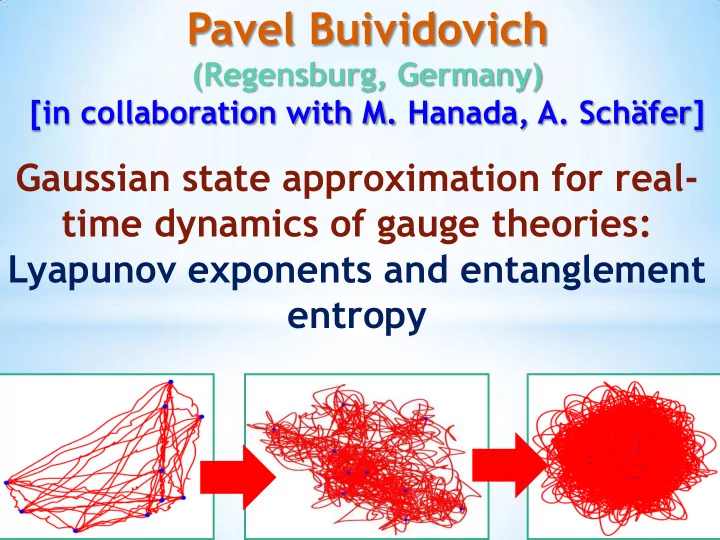
Pavel Buividovich (Regensburg, Germany) [in collaboration with M. Hanada, A. Schäfer] Gaussian state approximation for real- time dynamics of gauge theories: Lyapunov exponents and entanglement entropy

Motivation Glasma state at early stages of HIC Overpopulated gluon states Almost “classical” gauge fields Chaotic Classical Dynamics [Saviddy,Susskind …] Positive Lyapunov • exponents Gauge fields forget • initial conditions …but is it enough for Thermalization?

Motivation Thermalization for quantum systems? Quantum extension of Lyapunov • exponents - OTOCs <[P(0),X(t)] 2 > • Generation of entanglement between subsystems Timescales: quantum vs classical ?  QFT tools extremely limited beyond strong- field classic regime…  …Holography provides intuition

Bounds on chaos Reasonable physical assumptions Analyticity of OTOCs (QGP ~0.1 fm/c) [Maldacena Shenker Stanford’15] • Holographic models with black holes saturate the bound(e.g. SYK) • In contrast, for classical YM What happens at low T ???

Motivation N=1 Supersymmetric Yang-Mills in D=1+9: Reduce to a single point = BFSS matrix model [Banks, Fischler, Shenker, S usskind’1997] N x N hermitian Majorana-Weyl fermions, matrices N x N hermitian System of N D0 branes joined by open strings [Witten’96] : X i i μ = D0 brane positions • X ij μ = open string excitations •

Classical chaos and BH physics Stringy interpretation: • Dynamics of gravitating D0 branes • Thermalized state = black hole • Classical chaos = info scrambling Expected to saturate the MSS bound at low temperatures!

In this talk: Numerical attempt to look at the real-time dynamics of BFSS and bosonic matrix models Of course, not an exact simulation, but should be good at early times Approximating all states by Gaussians

Gaussian state approximation Simple example: Double-well potential Heisenberg equations of motion Also, for example

Next step: Gaussian Wigner function Assume Gaussian wave function at any t Simpler: Gaussian Wigner function For other correlators: use Wick theorem! Derive closed equations for x, p, σ xx , σ xp , σ pp

Origin of tunnelling Positive force even at x=0 (classical minimum) Quantum force causes classical trajectory to leave classical minimum

Gaussian state vs exact Schrödinger σ 2 =0.1 σ 2 =0.02 σ 2 =0.2 σ 2 =0.5 Early-time evolution OK • Tunnelling period qualitatively OK •

2D potential with flat directions (closer to BFSS model) Classic runaway along x=0 or y=0 Classically chaotic! We start with a Gaussian wave packet at distance f from the origin (away from flat directions)

Gaussian state vs exact Schrödinger

Gaussian state approximation  Is good for at least two classical Lyapunov times  Maps pure states to pure states  Allows to study entanglement  Closely related to semiclassics  Is better for chaotic than for regular systems [nlin/0406054]  Is likely safe in the large-N limit X Is not a unitary evolution

BFSS matrix model: Hamiltonian formulation a,b,c – su(N) Lie algebra indices Heisenberg equations of motion

GS approximatio for BFSS model CPU time ~ N^5 (double commutators) • RAM memory ~ N^4 • SUSY broken, unfortunately … •

Ungauging the BFSS model Gauge constraints • For Gaussian states we can only have a • weaker constraint We work with ungauged model • [Maldacena,Milekhin’1802.00428] (e.g. LGT with unit Polyakov loops) Ungauging preserves most of the • features of the original model [1802.02985]

Equation of state and temperature Consider mixed Gaussian states with • fixed energy E = <H> Maximize entropy w.r.t. <xx>,<pp> • Calculate temperature using • Can be done analytically using • rotational and SU(N) symmetries

“Thermal” initial conditions • At T=0 pure “ground” state with minimal <pp>,<xx> • At T>0 mixed states, interpret as mixture of pure states, shifted by “classical” coordinates with dispersion <xx>-<xx> 0 • Makes difference for non-unitary evolution • Fermions in ground state at fixed classical coordinates

Energy vs temperature MC data from [Berkowitz,Hanada, Rinaldi, Vranas, 1802.02985], we agree for pure gauge

<1/N Tr(X i 2 )> vs temperature MC data from [Berkowitz,Hanada, Rinaldi, Vranas, 1802.02985], we agree for pure gauge

Real-time evolution: <1/N Tr(X i 2 )> Wavepacket spread vs classical shrinking For BFSS <1/N Tr(X i 2 )> grows, instability?

Entanglement vs time Late-time saturation = information scrambling Entanglement entropy ~ subsystem size

Lyapunov distances vs time Early times: Very similar to classical dynamics Late times: significantly slower growth

Lyapunov vs entanglement: bosonic MM MSS: λ L 0~ T 1/4 λ L <2 π T Entanglement saturates much faster than Lyapunov time, at high T – classical Lyapunov

Bosonic MM vs BFSS MSS: λ L <2 π T ??? • No strong statements at low T: loss of SUSY • Non-chaotic confinement regime absent • Shortest timescale still for entanglement

Summary • Longer quantum Lyapunov times vs. classical, important for MSS bound • “Confining” regime non -chaotic • Full BFSS model chaotic at all T • “Scrambling” behavior for entanglement entropy • Entanglement timescale is the shortest • At high T governed by classic Lyapunov

Summary • Gaussian state approximation: ~V 2 scaling of CPU time for QCD/ Yang-Mills • Feasible on moderately large lattices • Quantum effects on thermalization? • Topological transitions in real time