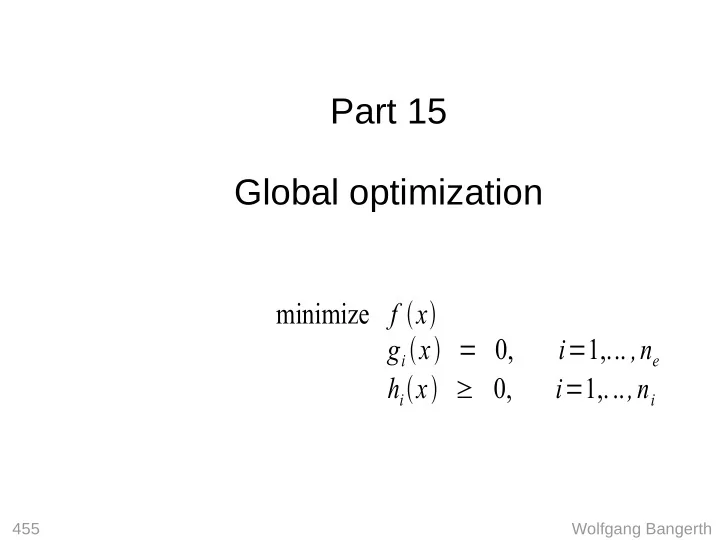
Part 15 Global optimization minimize f x g i x = 0, i = 1,... ,n - PowerPoint PPT Presentation

Part 15 Global optimization minimize f  x  g i  x  = 0, i = 1,... ,n e h i  x  ≥ 0, i = 1,... ,n i 455 Wolfgang Bangerth

Motivation What should we do when asked to find the (global) minimum of functions like this: f  x = 1 2  x 2 2  cos  x 1  cos  x 2  20  x 1 456 Wolfgang Bangerth

A naïve sampling approach Naïve approach: Sample at M -by- M points and choose the one with the smallest value. Alternatively: Start Newton's method at each of these points to get higher accuracy. Problem: If we have n variables, then we would have to start at M n points. This becomes prohibitive for large n ! 457 Wolfgang Bangerth

Monte Carlo sampling A better strategy (“Monte Carlo” sampling): ● Start with a feasible point x 0 ● For k=0,1,2,... : x t - Choose a trial point f  x t ≤ f  x k  x k  1 = x t - If then [ accept the sample] - Else: . draw a random number s in [0,1] . if exp [ − f  x t − f  x k  ] ≥ s T then x k  1 = x t [ accept the sample] else x k  1 = x k [ reject the sample] 458 Wolfgang Bangerth

Monte Carlo sampling Example: The first 200 sample points 459 Wolfgang Bangerth

Monte Carlo sampling Example: The first 10,000 sample points 460 Wolfgang Bangerth

Monte Carlo sampling Example: The first 100,000 sample points 461 Wolfgang Bangerth

Monte Carlo sampling Example: Locations and values of the first 10 5 sample points 462 Wolfgang Bangerth

Monte Carlo sampling Example: Values of the first 100,000 sample points Note: The exact minimal value is -1.1032... . In the first 100,000 samples, we have 24 with values f(x)<-1.103 . 463 Wolfgang Bangerth

Monte Carlo sampling How to choose the constant T : ● If T is chosen too small, then the condition exp [ − f  x t − f  x k  ] ≥ s, s ∈ U [ 0,1 ] T will lead to frequent rejections of sample points for which f(x) increases. Consequently, we will get stuck in local minima for long periods of time before we accept a sequence of steps that gets “us over the hump”. ● On the other hand, if T is chosen too large, then we will accept nearly every sample, irrespective of f(x t ) . Consequently, we will perform a random walk that is no more efficient than uniform sampling. 464 Wolfgang Bangerth

Monte Carlo sampling Example: First 100,000 samples, T =0.1 465 Wolfgang Bangerth

Monte Carlo sampling Example: First 100,000 samples, T =1 466 Wolfgang Bangerth

Monte Carlo sampling Example: First 100,000 samples, T =10 467 Wolfgang Bangerth

Monte Carlo sampling Strategy: Choose T large enough that there is a reasonable probability to get out of local minima; but small enough that this doesn't happen too often. f  x = 1 2  x 2 2  cos  x 1  cos  x 2  20  x 1 Example: For the difference in function value between local minima and saddle points is around 2. We want to choose T so that exp [ − f T ] ≥ s, s ∈ U [ 0,1 ] is true maybe 10% of the time. This is the case for T=0.87. 468 Wolfgang Bangerth

Monte Carlo sampling How to choose the next sample x t : ● If x t is chosen independently of x k then we just sample the entire domain, without exploring areas where f(x) is small. Consequently, we should choose x t “close” to x k . ● If we choose x t too close to x k we will have a hard time exploring a significant part of the feasible region. ● If we choose x t in an area around x k that is too large, then we don't adequately explore areas where f(x) is small. Common strategy: Choose n  x t = x k  y , y ∈ N  0, I  or U [− 1,1 ] where σ is a fraction of the diameter of the domain or the distance between local minima. 469 Wolfgang Bangerth

Monte Carlo sampling Example: First 100,000 samples, T =1, σ =0.05 470 Wolfgang Bangerth

Monte Carlo sampling Example: First 100,000 samples, T =1, σ =0.25 471 Wolfgang Bangerth

Monte Carlo sampling Example: First 100,000 samples, T =1, σ =1 472 Wolfgang Bangerth

Monte Carlo sampling Example: First 100,000 samples, T =1, σ =4 473 Wolfgang Bangerth

Monte Carlo sampling with constraints Inequality constraints: ● For simple inequality constraints, modify sample generation strategy to never generate infeasible trial samples ● For complex inequality constraints, always reject samples for which h i  x t  0 for at least one i 474 Wolfgang Bangerth

Monte Carlo sampling with constraints Inequality constraints: ● For simple inequality constraints, modify the sample generation strategy to never generate infeasible trial samples ● For complex inequality constraints, always reject samples: Q  x t ≤ Q  x k  x k  1 = x t - If then - Else: . draw a random number s in [0,1] . if exp [ − Q  x t − Q  x k  ] ≥ s T then x k  1 = x t else x k  1 = x k where Q  x =∞ if at least one h i  x  0, Q  x = f  x  otherwise 475 Wolfgang Bangerth

Monte Carlo sampling with constraints Equality constraints: ● Generate only samples that satisfy equality constraints ● If we have only linear equality constraints of the form g  x = Ax − b = 0 then one way to guarantee this is to generate samples using n − n e , y = N  0, I  or U [− 1,1 ] n − n e  x t = x k  Z y , y ∈ℝ where Z is the null space matrix of A , i.e. AZ=0 . 476 Wolfgang Bangerth

Monte Carlo sampling Theorem: Let A be a subset of the feasible region. Under certain k ∞ conditions on the sample generation strategy, then as we have − f ( x ) T dx number of samples x k ∈ A ∝ ∫ A e That is: Every region A will be adequately sampled over time. Areas around the global minimum will be better sampled than other regions. In particular, − f ( x ) fraction of samples x k ∈ A = 1 1 T dx + O ( √ N ) C ∫ A e 477 Wolfgang Bangerth

Monte Carlo sampling Remark: Monte Carlo sampling appears to be a strategy that bounces around randomly, only taking into account the values (not the derivatives ) of f(x) . However, that is not so if sample generation strategy and T are chosen carefully: Then we choose a new sample moderately close to the previous one, and we always accept it if f(x) is reduced, whereas we only sometimes accept it if f(x) is increased by this step. In other words: On average we still move in the direction of steepest descent! 478 Wolfgang Bangerth

Monte Carlo sampling Remark: Monte Carlo sampling appears to be a strategy that bounces around randomly, only taking into account the values (not the derivatives ) of f(x) . However, that is not so – because it compares function values. That said: One can accelerate the Monte Carlo method by choosing samples from a distribution that is biased towards the negative gradient direction if the gradient is cheap to compute. Such methods are sometimes called Langevin samplers . 479 Wolfgang Bangerth

Simulated Annealing Motivation: Particles in a gas, or atoms in a crystal have an energy that is on average in equilibrium with the rest of the system. At any given time, however, its energy may be higher or lower. In particular, the probability that its energy is E is − E k B T P  E  ∝ e Where k B is the Boltzmann constant. Likewise, probability that a particle can overcome an energy barrier of height ΔE is − E 1 if  E ≤ 0 P  E  E  E  ∝ min { 1, e k B T } = { k B T if  E  0 } −  E e This is exactly the Monte Carlo transition probability if we identify E = f k B 480 Wolfgang Bangerth

Simulated Annealing Motivation: In other words, Monte Carlo sampling is analogous to watching particles bounce around in a potential f(x) when driven by a gas at constant temperature. On the other hand, we know that if we slowly reduce the temperature of a system, it will end up in the ground state with very high probability. For example, slowly reducing the temperature of a melt results in a perfect crystal. (On the other hand, reducing the temperature too quickly results in a glass.) The Simulated Annealing algorithm uses this analogy by using the modified transition probability f  x t − f  x k  exp [ − ] ≥ s, s ∈ U [ 0,1 ] , T k  0 as k ∞ T k 481 Wolfgang Bangerth

Simulated Annealing Example: First 100,000 samples, σ =0.25 1 T = 1 T k = − 4 k 1  10 482 Wolfgang Bangerth

Simulated Annealing Example: First 100,000 samples, σ =0.25 1 T = 1 T k = − 4 k 1  10 24 samples with f(x)<-1.103 192 samples with f(x)<-1.103 483 Wolfgang Bangerth

Simulated Annealing 1 2 2  cos  x i  f  x = ∑ i = 1 x i Convergence: First 1,500 samples, 20 1 T = 1 T k = 1  0.005 k (Green line indicates the lowest function value found so far) 484 Wolfgang Bangerth

Simulated Annealing 1 10 2  cos  x i  f  x = ∑ i = 1 Convergence: First 10,000 samples, 20 x i 1 T = 1 T k = 1  0.0005 k (Green line indicates the lowest function value found so far) 485 Wolfgang Bangerth