Overcoming the curse of dimensionality: from nonlinear Monte Carlo - PowerPoint PPT Presentation

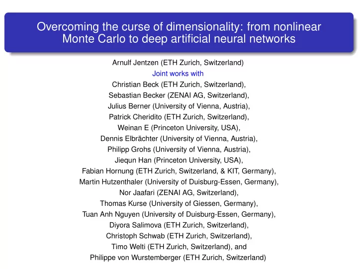
Overcoming the curse of dimensionality: from nonlinear Monte Carlo to deep artificial neural networks Arnulf Jentzen (ETH Zurich, Switzerland) Joint works with Christian Beck (ETH Zurich, Switzerland), Sebastian Becker (ZENAI AG, Switzerland), Julius Berner (University of Vienna, Austria), Patrick Cheridito (ETH Zurich, Switzerland), Weinan E (Princeton University, USA), Dennis Elbrächter (University of Vienna, Austria), Philipp Grohs (University of Vienna, Austria), Jiequn Han (Princeton University, USA), Fabian Hornung (ETH Zurich, Switzerland, & KIT, Germany), Martin Hutzenthaler (University of Duisburg-Essen, Germany), Nor Jaafari (ZENAI AG, Switzerland), Thomas Kurse (University of Giessen, Germany), Tuan Anh Nguyen (University of Duisburg-Essen, Germany), Diyora Salimova (ETH Zurich, Switzerland), Christoph Schwab (ETH Zurich, Switzerland), Timo Welti (ETH Zurich, Switzerland), and Philippe von Wurstemberger (ETH Zurich, Switzerland)

Computational problems from Financial Engineering (Evaluations of risks and financial products, XVA, optimal stopping), Operations Research (Optimal control, robots, game intelligence, optimal use of resources, formation of prices), Filtering (Chemical engineering, Kushner and Zakai equations) often require approximations for high-dimensional functions such as u : [ 0 , 1 ] d → R for d ∈ N large. Approximations methods such as finite element methods, finite differences, sparse grids suffer under the curse of dimensionality (Bellman 1957). Monte Carlo method based on Feynman-Kac formula: high-dimensional linear partial differential equations (PDEs) Deep BSDE method: Han, J, E 2017 PNAS , E, Han, J 2017 Comm. Math. Stat. , . . .

Theorem (Hutzenthaler, J, Kruse, Nguyen 2019) Let T , p , κ > 0 , let f : R → R be Lipschitz, ∀ d ∈ N let g d ∈ C ( R d , R ) and u d : [ 0 , T ] × R d → R be an at most poly. grow. solution of ∂ u d ∂ t = ∆ x u d + f ( u d ) u d ( 0 , · ) = g d , with assume | g d ( x ) | ≤ κ d κ ( 1 + � x � κ ) , let A l : R l → R l , l ∈ N , satisfy A l ( x 1 , . . . , x l ) = ( max { x 1 , 0 } , . . . , max { x l , 0 } ) , let n = 1 ( R l n × l n − 1 × R l n )) , N = ∪ L ∈ N ∪ l 0 ,..., l L ∈ N ( × L a , b = 1 C ( R a , R b ) satisfy for all L ∈ N , l 0 , . . . , l L ∈ N , let R : N → ∪ ∞ n = 1 ( R l n × l n − 1 × R l n ) , x 0 ∈ R l 0 , . . . , x L − 1 ∈ R l L − 1 Φ = (( W 1 , B 1 ) , . . . , ( W L , B L )) ∈ × L with ∀ n ∈ N ∩ ( 0 , L ): x n = A l n ( W n x n − 1 + B n ) that ( R Φ)( x 0 ) = W L x L − 1 + B L , let P : N → N be the number of parameters, and let ( G d ,ε ) d ∈ N , ε ∈ ( 0 , 1 ] ⊆ N satisfy P ( G d ,ε ) ≤ κ d κ ε − κ and | g d ( x ) − ( R G d ,ε )( x ) | ≤ εκ d κ ( 1 + � x � κ ) . Then ∃ ( U d ,ε ) d ∈ N ,ε ∈ ( 0 , 1 ] ⊆ N , c > 0 : ∀ d ∈ N , ε ∈ ( 0 , 1 ]: � 1 / p � � [ 0 , T ] × [ 0 , 1 ] d | u d ( y ) − ( R U d ,ε )( y ) | p dy P ( U d ,ε ) ≤ c d c ε − c . ≤ ε and Linear PDEs: Grohs, Hornung, J, von Wurstemberger 2018; Berner, Grohs, J 2018; Elbrächter, Grohs, J, Schwab 2018; J, Salimova, Welti 2018

n = 1 Z n , Full history recursive Multilevel-Picard method: Let T > 0, L , p ≥ 0, Θ = ∪ ∞ ∀ d ∈ N let g d ∈ C ( R d , R ) satisfy ∀ x ∈ R d : | g d ( x ) | ≤ L ( 1 + � x � p ) , let f : R → R be Lipschitz, let (Ω , F , P ) probab. sp., let W d ,θ : [ 0 , T ] × Ω → R d , d ∈ N , θ ∈ Θ , be i.i.d. Brownian motions, let S θ : [ 0 , T ] × Ω → R , θ ∈ Θ , i.i.d. continuous satisfying ∀ t ∈ [ 0 , T ] , θ ∈ Θ that S θ t is U [ t , T ] -distributed, assume that n , M : [ 0 , T ] × R d × Ω → R , d ,θ ( S θ ) θ ∈ Θ and ( W d ,θ ) θ ∈ Θ , d ∈ N are independent, let U n , M ∈ Z , θ ∈ Θ , d ∈ N , satisfy ∀ d , n , M ∈ N , θ ∈ Θ , t ∈ [ 0 , T ] , x ∈ R d : d ,θ d ,θ − 1 , M ( t , x ) = U 0 , M ( t , x ) = 0 and U M n d , ( θ, 0 , − m ) g d ( x + W ) d ,θ � T − t n , M ( t , x ) = U M n m = 1 � n − 1 M n − l � �� � ( T − t ) � d , ( θ, l , m ) S ( θ, l , m ) d , ( θ, l , m ) � + , x + W f U l , M M n − l t S ( θ, l , m ) − t t l = 0 m = 1 ��� � d , ( θ, l , m ) S ( θ, l , m ) d , ( θ, l , m ) � − ✶ N ( l ) f , x + W U l − 1 , M t S ( θ, l , m ) − t t d , 0 and ∀ d , n ∈ N let Cost d , n ∈ N be the comp. cost of U n , n ( 0 , 0 ) .

Then i) ∀ d ∈ N : there exists u d : [ 0 , T ] × R d → R at most polyn. grow. solution of ∂ u d ∂ t + 1 2 ∆ x u d + f ( u d ) = 0 u d ( T , · ) = g d with and ii) ∀ δ > 0 : there exist n : N × ( 0 , ∞ ) → N and C > 0 : ∀ d ∈ N , ε > 0 : n d ,ε , n d ,ε ( 0 , 0 ) | 2 �� 1 / 2 ≤ ε | u d ( 0 , 0 ) − U d , 0 � � E and Cost d , n d ,ε ≤ Cd 1 + p ( 1 + δ ) ε − ( 2 + δ ) . Extensions: Algorithms/Simulations/Proofs: Fully nonlinear PDEs (Beck, E, J 2018 JNS ), Optimal stopping (Becker, Cheridito, J 2018 JMLR ), Uniform errors (Beck, Becker, Grohs, Jaafari, J 2018), Semilinear PDEs/CVA (Hutzenthaler, J, von Wurstemberger 2019), . . .