Three Questions � Do (smallest) solutions always exist ? How to compute the ( smallest ) solution ? � How How to to compute compute the the ( (smallest smallest) ) solution solution ? ? � � How to justify that a solution is what we want ? � How How to to justify justify that that a a solution solution is is what what we we want want ? ? � � ������������������������������������������������������������������������������ ��������� �$
Knaster-Tarski Fixpoint Theorem Definitions: Let ( L , ⊑ ) be a partial order. � f : L → L is monotonic iff ∀ x,y ∈ L : x ⊑ y ⇒ f ( x ) ⊑ f ( y ). � x ∈ L is a fixpoint of f iff f ( x )= x . Fixpoint Theorem of Knaster-Tarski: Every monotonic function f on a complete lattice L has a least fixpoint lfp( f ) and a greatest fixpoint gfp( f ). More precisely , lfp( f ) = ⊓ { x ∈� L | f ( x ) ⊑ x } least pre-fixpoint gfp( f ) = ⊔ { x ∈� L | x ⊑ f ( x ) } greatest post-fixpoint
Knaster-Tarski Fixpoint Theorem ⊤ ⊤ ⊤ ⊤ L: pre-fixpoints of f gfp(f) fixpoints of f lfp(f) post-fixpoints of f ⊥ ⊥ ⊥ ⊥ Picture from: Nielson/Nielson/Hankin, Principles of Program Analysis
Smallest Solutions Always Exist � Define functional F : L n → L n from right hand sides of constraints such that: σ solution of constraint system iff σ pre-fixpoint of F � � Functional F is monotonic. � By Knaster-Tarski Fixpoint Theorem: F has a least fixpoint which equals its least pre-fixpoint. � ☺ ☺ ☺ ☺ ������������������������������������������������������������������������������ ��������� ��
Three Questions Do ( smallest ) solutions always exist ? � Do ( Do (smallest smallest) ) solutions solutions always always exist exist ? ? � � � How to compute the (smallest) solution ? How to justify that a solution is what we want ? � How How to to justify justify that that a a solution solution is is what what we we want want ? ? � � ������������������������������������������������������������������������������ ��������� �!
Workset-Algorithm W = ∅ ; { } forall ( v ) { A v [ ] =⊥ ; W = W ∪ v ; } program points A fin [ ] = init ; while W ≠ ∅ { v = Extract W ( ); forall ( , u s with e = ( , , ) u s v ) { edge t = f A v ( [ ]); e ⊑ if ¬ ( t A u [ ]) { ⊔ A u [ ] = A u [ ] t ; { } W = W ∪ u ; } } } ������������������������������������������������������������������������������ ��������� �%
Invariants of the Main Loop ⊑� a) A u [ ] MFP[ ] u f.a. prg. points u ⊒� b1) A fin [ ] init ⇒ ⊒ b2) v ∉ W [ ] A u f ( [ ]) f.a. edges A v e = ( , , ) u s v e If and when workset algorithm terminates: is a solution of the constraint system by b1)&b2) A ⇒ ⊒�� [ ] A u MFP u [ ] f.a. u ☺ ☺ ☺ ☺ �� Hence, with a): [ ] A u = MFP u [ ] f.a. u ������������������������������������������������������������������������������ ��������� �&
How to Guarantee Termination � Lattice ( L , ⊑ ) has finite heights ⇒ algorithm terminates after at most #prg points � (heights(L)+1) iterations of main loop � Lattice ( L , ⊑ ) has no infinite ascending chains ⇒ algorithm terminates � Lattice ( L , ⊑ ) has infinite ascending chains: ⇒ algorithm may not terminate; use widening operators in order to enforce termination ������������������������������������������������������������������������������ ��������� �
[Cousot] Widening Operator ▽ : L × L → L is called a widening operator iff 1) ∀ x,y ∈ L : x ⊔ y ⊑ x ▽ y 2) for all sequences ( l n ) n , the (ascending) chain ( w n ) n w 0 = l 0 , w i +1 = w i ▽ l i+1 for i > 0 stabilizes eventually.
Workset-Algorithm with Widening W = ∅ ; { } forall ( v ) { A v [ ] =⊥ ; W = W ∪ v ; } program points A fin [ ] = init ; while W ≠ ∅ { v = Extract W ( ); forall ( , u s with e = ( , , ) u s v ) { edge t = f A v ( [ ]); e ⊑ if ¬ ( t A u [ ]) { ▽ A u [ ] = A u [ ] t ; { } W = W ∪ u ; } } } ������������������������������������������������������������������������������ ��������� �#
Invariants of the Main Loop ⊑� a) A u [ ] MFP[ ] u f.a. prg. points u ⊒� b1) A fin [ ] init ⇒ ⊒ b2) v ∉ W [ ] A u f ( [ ]) f.a. edges A v e = ( , , ) u s v e With a widening operator we enforce termination but we loose invariant a ) . Upon termination, we have: is a solution of the constraint system by b1)&b2) A ⇒ ⊒�� [ ] A u MFP u [ ] f.a . u � � � � Compute a sound upper approximation (only) ! ������������������������������������������������������������������������������ ��������� �$
Example of a Widening Operator: Interval Analysis The goal Find save interval for the values of program variables, e.g. of i in: for (i=0; i<42; i++) if (0<=i and i<42) { A1 = A+i; M[A1] = i; } ☺ ..., e.g., in order to remove the redundant array range check.
Example of a Widening Operator: Interval Analysis The lattice... ( ) ⊑ { } ( ) ℤ { } ℤ { } { } L , = [ , ] | l u l ∈ ∪ −∞ , u ∈ ∪ +∞ , l ≤ u ∪ ∅ , ⊆ ... has infinite ascending chains, e.g.: [0,0] ⊂ [0,1] ⊂ [0,2] ⊂ ... A widening operator: ▽ [ , l u ] [ , l u ] = [ , l u ], where 0 0 1 1 2 2 l if l ≤ l u if u ≥ u 0 0 1 0 0 1 l = and u = 2 2 −∞ otherwise +∞ otherwise A chain of maximal length arising with this widening operator: ∅ ⊂ [3,7] ⊂ [3, +∞ ⊂ −∞ +∞ ] [ , ]
Analyzing the Program with the Widening Operator � ⇒ Result is far too imprecise ! Example taken from: H. Seidl, Vorlesung „Programmoptimierung“
Remedy 1: Loop Separators � Apply the widening operator only at a „ loop separator “ (a set of program points that cuts each loop). � We use the loop separator {1} here. Identify condition at edge from 2 to 3 as redundant ! ☺ ⇒
Remedy 2: Narrowing � Iterate again from the result obtained by widening --- Iteration from a prefix-point stays above the least fixpoint ! --- ☺ ⇒ We get the exact result in this example (but not guaranteed) !
Remarks � Can use a work-list instead of a work-set � Special iteration strategies in special situations � Semi-naive iteration ������������������������������������������������������������������������������ ��������� !&
Recall: Specifying Live Variables Analysis by a Constraint System Compute (smallest) solution over ( L , ⊑ ) = (P(Var), ⊆ ) of: ⊒ A fin [ ] init , for fin , the termination node ⊒ A u [ ] f ( [ ]), A v for each edge e = ( , , ) u s v e where init = Var, f e :P(Var) → P(Var), f e ( x ) = x \ kill e ∪ gen e , with kill e = variables assigned at e � gen e = variables used in an expression evaluated at e �
Recall: Questions � Do (smallest) solutions always exist ? � How to compute the (smallest) solution ? � How to justify that a solution is what we want ? ������������������������������������������������������������������������������ ��������� !"
Three Questions Do ( smallest ) solutions always exist ? � Do ( Do (smallest smallest) ) solutions solutions always always exist exist ? ? � � How to compute the ( smallest ) solution ? � How How to to compute compute the the ( (smallest smallest) ) solution solution ? ? � � � How to justify that a solution is what we want ? � MOP vs MFP-solution � Abstract interpretation ������������������������������������������������������������������������������ ��������� !#
Three Questions Do ( smallest ) solutions always exist ? � Do ( Do (smallest smallest) ) solutions solutions always always exist exist ? ? � � How to compute the ( smallest ) solution ? � How How to to compute compute the the ( (smallest smallest) ) solution solution ? ? � � � How to justify that a solution is what we want ? � MOP vs MFP-solution Abstract interpretation � Abstract Abstract interpretation interpretation � � ������������������������������������������������������������������������������ ��������� !$
Assessing Data Flow Frameworks Execution Abstraction MOP-solution Semantics sound? sound? MFP-solution how precise? precise? ������������������������������������������������������������������������������ ��������� %�
Live Variables ∅ ∅ {y} x := 17 y := 17 x := 42 y := x+y x := 10 x := y+1 x := x+1 y := 11 x := y+1 infinitely many such paths out(x) = ∅ ∪ = MOP[ ] v { } y { } y
Meet-Over-All-Paths Solution (MOP) � Forward Analysis ⊔ � = MOP[ ] : u F ( init ) ∈ p Paths[ entry u , ] p � Backward Analysis ⊔ � = MOP[ ] : u F ( init ) ∈ p Paths[ , u exit ] p � Here: „Join-over-all-paths“; MOP traditional name ������������������������������������������������������������������������������ ��������� %�
Coincidence Theorem Definition: A framework is positively-distributive if f( ⊔ X)= ⊔ { f(x) | x ∈ X} for all ∅ ≠ X ⊆ L, f ∈ F. Theorem: For any instance of a positively-distributive framework: MOP[u] = MFP[u] for all program points u (if all program points reachable). Remark: A framework is positively-distributive if a) and b) hold: (a) it is distributive: f(x ⊔ y) = f(x) ⊔ f(y) f.a. f ∈ F, x,y ∈ L. (b) it is effective: L does not have infinite ascending chains . Remark: All bitvector frameworks are distributive and effective. ������������������������������������������������������������������������������ ��������� %!
Lattice for Constant Propagation ⊤ unknown value . . . -2 -1 0 1 2 . . . ⊥ ℤ ⊤ ρ ρ → ∪ ∪ lattice : L { | : Var ( { })} { } �������⊑ �� ⊑ ⊥ ρ ρ ⇔ ρ = ∨ : ' : ⊑ ⊥ ρ ρ ≠ ∧∀ ρ ρ ( , ' x : ( ) x '( )) x
ρ ρ ρ ( ( ), x ( ), y ( )) z x := 17 x := 2 x := 3 y := 3 y := 2 z := x+y (2,3,5) (3,2,5) ⊤ ⊤ out(x) = MOP[ ] ( v , ,5) ������������������������������������������������������������������������������ ��������� %&
ρ ρ ρ ( ( ), x ( ), y ( )) z x := 17 ( ⊤ , ⊤ , ⊤ ) x := 2 x := 3 (2, ⊤ , ⊤ ) (3, ⊤ , ⊤ ) y := 3 y := 2 (2,3, ⊤ ) (3,2, ⊤ ) ( ⊤ , ⊤ , ⊤ ) z := x+y ⊤ ⊤ ⊤ = M FP[ ] ( v , , ) ( ⊤ , ⊤ , ⊤ ) ⊤ ⊤ out(x) = MOP[ ] ( v , ,5) ������������������������������������������������������������������������������ ��������� %
Correctness Theorem Definition: A framework is monotone if for all f ∈ F, x,y ∈ L: x ⊑ y f(x) ⊑ f(y) . ⇒ Theorem: In any monotone framework: MOP[u] ⊑ MFP[u] for all program points u. Remark: ☺ ☺ ☺ ☺ Any "reasonable" framework is monotone. ������������������������������������������������������������������������������ ��������� %"
Assessing Data Flow Frameworks Execution Abstraction MOP-solution Semantics sound sound MFP-solution precise, if distrib. ������������������������������������������������������������������������������ ��������� %#
Where Flow Analysis Looses Precision Execution MOP MFP Widening semantics Potential loss of precision ������������������������������������������������������������������������������ ��������� %$
Three Questions Do ( smallest ) solutions always exist ? � Do ( Do (smallest smallest) ) solutions solutions always always exist exist ? ? � � How to compute the ( smallest ) solution ? � How How to to compute compute the the ( (smallest smallest) ) solution solution ? ? � � � How to justify that a solution is what we want ? MOP vs MFP - solution � MOP MOP vs vs MFP MFP- -solution solution � � � Abstract interpretation ������������������������������������������������������������������������������ ��������� &�
Abstract Interpretation constraint system for constraint system for Replace Reference Semantics Analysis concrete operators o on concrete lattice (D, ⊑ ) on abstract lattice (D # , ⊑ # ) by abstract operators o # MFP # MFP Often used as reference semantics: sets of reaching runs: � (D, ⊑ ) = (P(Edges * ), ⊆ ) or (D, ⊑ ) = (P(Stmt * ), ⊆ ) sets of reaching states („ collecting semantics“ ): � (D, ⊑ ) = (P( Σ * ), ⊆ ) with Σ = Var → Val ������������������������������������������������������������������������������ ��������� &�
Abstract Interpretation constraint system for constraint system for Replace Reference Semantics Analysis concrete operators o on concrete lattice (D, ⊑ ) on abstract lattice (D # , ⊑ # ) by abstract operators o # MFP # MFP Assume a universally-disjunctive abstraction function α : D → D # . Correct abstract interpretation: Show α (o(x 1 ,...,x k )) ⊑ # o # ( α (x 1 ),..., α (x k )) f.a. x 1 ,...,x k ∈ L, operators o Then α (MFP[u]) ⊑ # MFP # [u] f.a. u Correct and precise abstract interpretation: Show α (o(x 1 ,...,x k )) = o # ( α (x 1 ),..., α (x k )) f.a. x 1 ,...,x k ∈ L, operators o Then α (MFP[u]) = MFP # [u] f.a. u Use this as a guideline for designing correct (and precise) analyses ! ������������������������������������������������������������������������������ ��������� &�
Abstract Interpretation Constraint system for reaching runs: { } R st [ ] ⊇ ε , for , the start node st { } R v [ ] ⊇ R u [ ] ⋅ e , for each edge e = ( , , ) u s v Operational justification: Let R[u] be components of smallest solution over P(Edges *) . Then op r R u [ ] = R [ ] u = { r ∈ Edges *| st → u } for all u def Prove: a) R op [u] satisfies all constraints (direct) ⇒ R[u] ⊆ R op [u] f.a. u b) w ∈ R op [u] ⇒ w ∈ R[u] (by induction on |w|) ⇒ R op [u] ⊆ R[u] f.a. u
Abstract Interpretation Constraint system for reaching runs: { } R st [ ] ⊇ ε , for st , the start node { } R v [ ] ⊇ R u [ ] ⋅ e , for each edge e = ( , , ) u s v Derive the analysis: Replace { ε } by init ( • ) � { � e � } by f e Obtain abstracted constraint system: ⊒ # R st [ ] init , for st , the start node ⊒ # # R v [ ] f R u ( [ ]), for each edge e = ( , , ) u s v e
Abstract Interpretation MOP-Abstraction: Define α MOP : P(Edges *) → L by ⊔ { } � α MOP ( R ) = f init ( ) | r ∈ R where f = Id f , = f f r ε e s s e ⋅ Remark: For all transfer functions f e are monotone, the abstraction is correct: α Μ OP (R[u]) ⊑ R # [u] f.a. prg. points u If all transfer function f e are universally-distributive, the abstraction is correct and precise: α Μ OP (R[u]) = R # [u] f.a. prg. points u ☺ ☺ ☺ ☺ Justifies MOP vs. MFP theorems ( cum grano salis ).
Overview Introduction � Fundamentals of Program Analysis � Excursion 1 Interprocedural Analysis � Excursion 2 Analysis of Parallel Programs � Excursion 3 Appendix Conclusion � ������������������������������������������������������������������������������ ��������� &
Challenges for Automatic Analysis � Data aspects: infinite number domains � dynamic data structures (e.g. lists of unbounded length) � pointers � ... � � Control aspects: recursion � concurrency � creation of processes / threads � synchronization primitives (locks, monitors, communication stmts ...) � ... � ⇒ ⇒ ⇒ ⇒ infinite/unbounded state spaces ������������������������������������������������������������������������������ ��������� &"
Classifying Analysis Approaches control aspects data aspects analysis techniques ������������������������������������������������������������������������������ ��������� &#
(My) Main Interests of Recent Years Data aspects: algebraic invariants over Q , Z , Z m ( m = 2 n ) in sequential programs, � partly with recursive procedures invariant generation relative to Herbrand interpretation � Control aspects: recursion � concurrency with process creation / threads � synchronization primitives, in particular locks/monitors � Technics: fixpoint-based � automata-based � (linear) algebra � syntactic substitution-based techniques � ... �
Overview Introduction � Fundamentals of Program Analysis � Excursion 1 Interprocedural Analysis � Excursion 2 Analysis of Parallel Programs � Excursion 3 Appendix Conclusion � ������������������������������������������������������������������������������ ��������� �
A Note on Karr´s Algorithm Markus Müller-Olm FernUniversität Hagen (on leave from Universität Dortmund) Joint work with Helmut Seidl (TU München) ICALP 2004, Turku, July 12-16, 2004
What this Excursion is About… 0 x 1 :=1 x 2 :=1 x 3 :=1 1 x 1 :=x 1 +1 x 2 :=2x 2 -2x 1 +5 x 3 :=x 3 +x 2 2 2 x 3 = x 1 x 2 = 2x 1 -1
Affine Programs � Basic Statements: � affine assignments: x 1 := x 1 -2x 3 +7 � unknown assignments: x i := ? → abstract too complex statements � Affine Programs: � control flow graph G=(N,E,st), where � N finite set of program points � E ⊆ N × Stmt × N set of edges � st ∈ N start node � Note: non-deterministic instead of guarded branching
The Goal: Precise Analysis Given an affine program, determine for each program point � all valid affine relations: a 0 + ∑ a i x i = 0 a i ∈ � 5x 1 +7x 2 -42=0 More ambitious goal: � determine all valid polynomial relations (of degree � d): p ∈ � [x 1 ,…,x n ] p(x 1 ,…,x k ) = 0 2 +7x 3 3 =0 5x 1 x 2
Applications of Affine (and Polynomial) Relations � Data-flow analysis: � definite equalities: x = y � constant detection: x = 42 � discovery of symbolic constants: x = 5yz+17 xy+42 = y 2 +5 � complex common subexpressions: � loop induction variables � Program verification � strongest valid affine (or polynomial) assertions (cf. Petri Net invariants)
[Karr, 1976] Karr´s Algorithm � Determines valid affine relations in programs. � Idea: Perform a data-flow analysis maintaining for each program point a set of affine relations, i.e., a linear equation system. � Fact: Set of valid affine relations forms a vector space of dimension at most k +1, where k = #program variables. ⇒ can be represented by a basis. ⇒ forms a complete lattice of height k+1.
Deficiencies of Karr´s Algorithm � Basic operations are complex „non-invertible“ assignments � union of affine spaces � � O( n � k 4 ) arithmetic operations n size of the program � k number of variables � � Numbers may have exponential length
Our Contribution � Reformulation of Karr´s algorithm: basic operations are simple � O( n � k 3 ) arithmetic operations � numbers stay of polynomial length: O( n � k 2 ) � Moreover: generalization to polynomial relations of bounded degree � show, algorithm finds all affine relations in „affine programs“ � � Ideas: represent affine spaces by affine bases instead of lin. eq. syst. � use semi-naive fixpoint iteration � keep a reduced affine basis for each program point during fixpoint � iteration
Affine Basis
Concrete Collecting Semantics Smallest solution over subsets of � k of: ℚ k V st [ ] ⊇ V v [ ] ⊇ f V u ( [ ]) , for each edge ( , , ) u s v s where { ֏ } f ( X ) = x x [ t x ( )] | x ∈ X x : = t i i { } ֏ ℚ f ( X ) = x x [ c ] | x ∈ X c , ∈ x : ? = i i First goal: compute affine hull of V [ u ] for each u .
Abstraction Affine hull: = ∑ ∑ { } ℚ aff X ( ) λ x | x ∈ X , λ ∈ , λ = 1 i i i i i The affine hull operator is a closure operator: ⇒ aff X ( ) ⊇ X aff aff X , ( ( )) = X , X ⊆ Y aff X ( ) ⊆ aff Y ( ) Affine subspaces of Q k ordered by set inclusion ⇒ form a complete lattice: ( ) { } ⊑ ℚ k ( , ) D = X ⊆ | aff X ( ) = X , ⊆ . Affine hull is even a precise abstraction: Lemma : ( f aff X ( )) = aff f ( ( X )). s s
Abstract Semantics Smallest solution over (D, ⊑ ) of: ⊒ # ℚ k V [ st ] ⊒ # # V [ ] v f V ( [ ]) , u for each edge ( , , ) u s v s # Le mma : V [ ] u = aff V u ( [ ]) for all progr am points u.
Basic Semi-naive Fixpoint Algorithm forall ( v ∈ N ) G v [ ] = ∅ ; G st [ ] {0, e ,..., e }; = 1 k W = {( st ,0),( st e , ),...,( st e , )}; 1 k while W ≠ ∅ { ( , ) u x = Extract W ( ); forall ( , s v with ( , , ) u s v ∈ E ) { � � t = s x ; if ( t ∉ aff G v ( [ ])) { { } G v [ ] = G v [ ] ∪ t ; { } W = W ∪ ( , ) ; v t } } }
Example 0 1 0 0 0 , 0 , 1 , 0 0 0 0 0 1 x 1 :=1 x 2 :=1 x 3 :=1 1 2 3 4 1 2 3 1 3 5 7 ∈ aff 1 , 3 , 5 1 1 4 9 16 1 4 9 x 1 :=x 1 +1 x 2 :=2x 2 -2x 1 +5 x 3 :=x 3 +x 2 2 3 4 3 2 5 7 4 9 16
Correctness Theore m : a) Algorithm terminates after at most nk + n iterations of the loop, where n = N and is the number of variables. k # b) For all v ∈ N , we have aff G ( [ ]) v = V [ v ] . fin Invariants for b) I1: ∀ ∈ v N G v : [ ] ⊆ V v [ ] and ( , ) ∀ u x ∈ W : x ∈ V u [ ]. � � ( ) { } ⊒ I2: (u,s,v) ∀ ∈ E: aff G v [ ] ∪ s x | ( , ) u x ∈ W f aff G u ( ( [ ]). s
Complexity Theo re m : # a) The affine hulls V [ ] u = aff V u ( [ ]) can be computed in time 3 O( n k ⋅ ), where n = | N | + | E |. b) In this computation only arithmetic operations on numbers 2 with O( n k ⋅ ) bits are u sed . Store diagonal basis for membership tests. Propagate original vectors.
Point + Linear Basis
Example 0 1 0 0 0 , 0 , 1 , 0 0 0 0 0 1 x 1 :=1 x 2 :=1 x 3 :=1 1 0 1 2 3 4 1 2 0 2 , 0 1 3 5 2 4 0 7 1 0 2 1 4 9 3 8 0 16 x 1 :=x 1 +1 x 2 :=2x 2 -2x 1 +5 x 3 :=x 3 +x 2 2 3 4 1 2 1 0 3 2 5 7 2 4 2 , 0 4 9 16 5 12 0 2
Determining Affine Relations Lemm a a : is valid for X ⇔ a is va lid for aff X ( ). ⇒ suffices to determine the affine relations valid for affine bases; can be done with a linear equation system! Theorem : a) The vector spaces of all affine relations valid at the program 3 points of an affine program can be computed in time O( n k ⋅ ). b) This computation performs arithmetic operatio ns on int egers 2 with O( n k ⋅ ) bits only.
Example a + a x + a x + a x = 0 is valid at 2 0 1 1 2 2 3 3 a + 2 a + 3 a + 4 a = 0 0 1 2 3 ⇔ 1 a + 2 a = 0 1 2 2 a = 0 3 0 x 1 :=1 ⇔ a = a , a = − 2 a , a = 0 0 2 1 2 3 x 2 :=1 x 3 :=1 ⇒ 2 x − x − 1 is valid at 2 1 2 1 x 1 :=x 1 +1 x 2 :=2x 2 -2x 1 +5 x 3 :=x 3 +x 2 2 3 4 1 0 3 2 5 7 2 , 0 4 9 16 0 2
Also in the Paper � Non-deterministic assignments � Bit length estimation � Polynomial relations � Affine programs + affine equality guards validity of affine relations undecidable � ������������������������������������������������������������������������������ ��������� #�
End of Excursion 1
(Optimal) Program Analysis of Sequential and Parallel Programs Markus Müller-Olm Westfälische Wilhelms-Universität Münster, Germany 3rd Summer School on Verification Technology, Systems, and Applications Luxemburg, September 6-10, 2010
Overview Introduction � Fundamentals of Program Analysis � Excursion 1 Interprocedural Analysis � Excursion 2 Analysis of Parallel Programs � Excursion 3 Appendix Conclusion � ������������������������������������������������������������������������������ ��������� #%
Interprocedural Analysis Main: P: procedures c:=a+b c:=a+b P() Q() call edges R() Q: R: a:=7 c:=a+b a:=7 c:=a+b P() R() recursion
Running Example: (Definite) Availability of the single expression a+b The lattice: false false a+b not available c:=a+b true a+b available true Initial value: false a:=7 c:=c+3 false true c:=a+b false true a:=42 false
Intra-Procedural-Like Analysis Conservative assumption: procedure destroys all information; information flows from call node to entry point of procedure Main: The lattice: st M false false c:=a+b true P: true u 1 true false st P P() λ x. false c:=a+b false u 2 r P true a:=7 false u 3 P() λ x. false � � � � false r M
Context-Insensitive Analysis Conservative assumption: Information flows from each call node to entry of procedure and from exit of procedure back to return point Main: The lattice: st M false false c:=a+b true P: true u 1 true false st P P() c:=a+b true u 2 r P true a:=7 false u 3 P() ☺ ☺ ☺ ☺ true r M
Context-Insensitive Analysis Conservative assumption: Information flows from each call node to entry of procedure and from exit of procedure bac to return point Main: The lattice: st M false false c:=a+b true P: true u 1 true false st P P() false true u 2 r P true false a:=7 false u 3 P() � � � � r M false
Recall: Abstract Interpretation Recipe constraint system for constraint system for Replace Reference Semantics Analysis concrete operators o on concrete lattice (D, ⊑ ) on abstract lattice (D # , ⊑ # ) by abstract operators o # MFP # MFP Assume a universally-disjunctive abstraction function α : D → D # . Correct abstract interpretation: Show α (o(x 1 ,...,x k )) ⊑ # o # ( α (x 1 ),..., α (x k )) f.a. x 1 ,...,x k ∈ L, operators o Then α (MFP[u]) ⊑ # MFP # [u] f.a. u Correct and precise abstract interpretation: Show α (o(x 1 ,...,x k )) = o # ( α (x 1 ),..., α (x k )) f.a. x 1 ,...,x k ∈ L, operators o Then α (MFP[u]) = MFP # [u] f.a. u Use this as a guideline for designing correct (and precise) analyses ! ������������������������������������������������������������������������������ ��������� $�
Example Flow Graph Main: The lattice: st M false e 0 : c:=a+b true P: u 1 st P e 1 : P() e 4 : c:=a+b u 2 r P e 2 : a:=7 u 3 e 3 : P() r M
Let‘s Apply Our Abstract Interpretation Recipe: Constraint System for Feasible Paths Operational justification: { ∗ r } | st S u ( ) = r ∈ Edges → u for all in procedure u p p { ∗ r } | st S p ( ) = r ∈ Edges → ε for all procedures p p { } ∗ r | ∃ w ∈ Nodes ∗ st R u ( ) = r ∈ Edges : → uw for all u Main Same-level runs : S p ( ) ⊇ S r ( ) r return point of p p p { } S st ( ) ⊇ ε st entry point of p p p { } S v ( ) ⊇ S u ( ) ⋅ e e = ( , , ) base edge u s v S(v) ⊇ S u ( ) ⋅ S p ( ) e = ( , , ) call edge u p v Reaching runs: { } R st ( ) ⊇ ε st entry point of Main Main Main { } R v ( ) ⊇ R u ( ) ⋅ e e = ( , , ) basic e u s v dg e R v ( ) ⊇ R u ( ) ⋅ S p ( ) e = ( , , ) call edge u p v R st ( ) ⊇ R u ( ) e = ( , , ) call ed u p v ge, st entry point of p p p
Context-Sensitive Analysis Idea : Phase 1: Compute summary information for each procedure... ... as an abstraction of same-level runs Phase 2: Use summary information as transfer functions for procedure calls... ... in an abstraction of reaching runs Classic approaches for summary informations: 1) Functional approach: [Sharir/Pnueli 81, Knoop/Steffen: CC´92] Use (monotonic) functions on data flow informations ! 2) Relational approach: [Cousot/Cousot: POPL´77] Use relations (of a representable class) on data flow informations ! 3) Call string approach: [Sharir/Pnueli 81], [Khedker/Karkare: CC´08] Analyse relative to finite portion of call stack !
Formalization of Functional Approach Abstractions: ∗ Abstract same-level runs with α :Edges → ( L → L ) : Funct ⊔ { } | r ∈ R ∗ α ( R ) = f for R ⊆ Edges Func t r ∗ Abstract reaching runs with α : Edges → L : M P O ⊔ { } | r ∈ R ∗ α ( R ) = f init ( ) for R ⊆ Edge s MOP r 1. Phase: Compute summary informations, i.e., functions : ⊒ # # S ( ) p S ( r ) r return point of p p p ⊒ # S ( st ) id st entry point of p p p ⊒ # # � # S ( ) v f S ( ) u e = ( , , ) base edge u s v e ⊒ � # # # S (v) S ( ) p S ( ) u e = ( , , ) call edge u p v 2. Phase: Use summary informations; compute on data flow informations: ⊒ # R ( st ) init st entry point of Main Main Main ⊒ # # # R ( ) v f ( R ( ) u ) e = ( , , ) basic edge u s v e ⊒ # # # R ( ) v S ( ) p R ( ( ) u ) e = ( , , ) call edg u p v e ⊒ # # R ( st ) R ( ) u e = ( , , ) call edge, u p v st entry point of p p p
Functional Approach Theorem: Correctness: For any monotone framework: α MOP (R[ u ]) ⊑ R # [ u ] f.a. u Completeness: For any universally-distributive framework: α MOP (R[ u ]) = R # [ u ] f.a. u Alternative condition: framework positively-distributive & all prog. point dyn. reachable Remark: a) Functional approach is effective, if L is finite... b) ... but may lead to chains of length up to | L | � height(L) at each program point (in general). ������������������������������������������������������������������������������ ��������� $&
Functional Approach for Availability of Single Expression Problem Observations: false Just three montone functions on lattice L : true λ x . false λ k (ill) λ λ λ λ x . x λ λ i (gnore) λ x . true λ λ λ g (enerate) Functional composition of two such functions f , g : L → L : f if h = i = � h f { } h i f h ∈ g , k Analogous: precise interprocedural analysis for ☺ ☺ ☺ ☺ all (separable) bitvector problems in time linear in program size.
Context-Sensitive Analysis, 1. Phase the lattice: Main: i i P: k g c:=a+b g c:=a+b i i g P() Q() g g i R() i k i Q: g R: k g a:=7 c:=a+b k g a:=7 c:=a+b k g k g P() R() g k g
Context-Sensitive Analysis, 2. Phase the lattice: Main: false i true false P: false g g true true false true true P() Q() true false true false R() true k Q: true g false R: k g k g false true false false true P() R() true false true
Functional Approach Theorem: Correctness: For any monotone framework: α MOP (R[ u ]) ⊑ R # [ u ] f.a. u Completeness: For any universally-distributive framework: α MOP (R[ u ]) = R # [ u ] f.a. u Alternative condition: framework positively-distributive & all prog. point dyn. reachable Remark: � � � � a) Functional approach is effective, if L is finite ... b) ... but may lead to chains of length up to | L | � height(L) at each program point. ������������������������������������������������������������������������������ ��������� ���
Overview Introduction � Fundamentals of Program Analysis � Excursion 1 Interprocedural Analysis � Excursion 2 Analysis of Parallel Programs � Excursion 3 Appendix Conclusion � ������������������������������������������������������������������������������ ��������� ���
Recommend
More recommend
Unleash a World of Digital Possibilities—Browse, Share, and Explore Content Without Boundaries