Optimal Portfolio Application with Double-Uniform Jump Model Floyd - - PowerPoint PPT Presentation

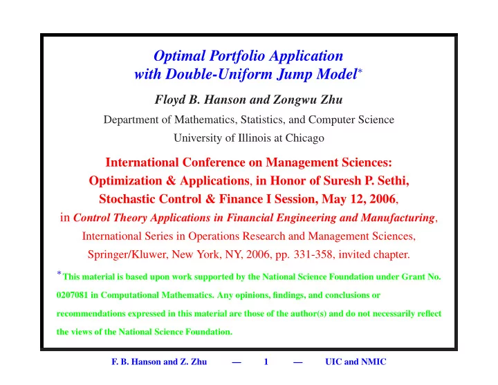
Optimal Portfolio Application with Double-Uniform Jump Model∗

Floyd B. Hanson and Zongwu Zhu

Department of Mathematics, Statistics, and Computer Science University of Illinois at Chicago

International Conference on Management Sciences: Optimization & Applications, in Honor of Suresh P. Sethi, Stochastic Control & Finance I Session, May 12, 2006, in Control Theory Applications in Financial Engineering and Manufacturing,

International Series in Operations Research and Management Sciences, Springer/Kluwer, New York, NY, 2006, pp. 331-358, invited chapter.

∗This material is based upon work supported by the National Science Foundation under Grant No. 0207081 in Computational Mathematics. Any opinions, findings, and conclusions or recommendations expressed in this material are those of the author(s) and do not necessarily reflect the views of the National Science Foundation.

• F. B. Hanson and Z. Zhu

— 1 — UIC and NMIC

Overview

• 1. Introduction.
• 2. Log-Return Double-Uniform Amplitude Jump-Diffusion Density.
• 3. Jump-Diffusion Parameter Estimation.
• 4. Application to Optimal Portfolio and Consumption Policies.
• Absorbing Boundary Condition at Zero Wealth.
• Non-Negativity of Wealth and Jump Distributions.
• Regular Control Policies.
• Optimal Control Policy Results.
• 5. Conclusions.
• F. B. Hanson and Z. Zhu

— 2 — UIC and NMIC

• 1. Introduction

1.1 Background:

• Merton’s 1971 pioneering J.E.T. paper on the optimal portfolio and

consumption problem for geometric diffusions used HARA (hyperbolic absolute risk-aversion) utility. However, there were errors, in particular with the bankruptcy boundary conditions and vanishing consumption, some errors were due to the HARA model. See also Merton’s 1969 lifetime portfolio paper in R.E.&S.

• Merton’s optimal portfolio errors are throughly discussed in the

seminal collection of papers with coauthors in Sethi’s bankruptcy book in 1997. See his introduction, the KLS(ethi)S M.O.R. 1986 paper and the J.E.T. 1988 paper with Taksar.

• F. B. Hanson and Z. Zhu

— 3 — UIC and NMIC

1.2 Market Jump Properties:

• Statistical evidence that jumps are significant in financial markets:

– Stock and Option Prices in Ball and Torous (’85); – Capital Asset Pricing Model in Jarrow and Rosenfeld (’84); – Foreign Exchange and Stocks in Jorion (’89).

• Log-return market distributions usually skewed negative,

η3 ≡ M3/(M2)1.5 < 0, if data time interval sufficiently long, compared to the skew-less normal distribution.

• Log-return market distributions usually leptokurtic,

η4 ≡ M4/(M2)2 > 3, i.e., more peaked than normal.

• Log-return market distribution have fatter or heavier tails than the

normal distribution’s exponentially small tails.

• Time-dependence of rate coefficients is important, i.e., non-constant

coefficients are important; and stochastic volatility.

• F. B. Hanson and Z. Zhu

— 4 — UIC and NMIC

1.3 Jump-Diffusion Models:

• Merton (J.F.E., 1976) in his pioneering jump-diffusion option

pricing model used IID log-normally distributed jump-amplitudes with a compound Poisson process. Other authors have also used the normal jump-applitude model.

• Kou (Mgt.Sci. 2002, and 2004 with Wang) used the IID

log-double-exponential (Laplace) for option pricing.

• Hanson and Westman (2001-2004) have a number of optimal

portfolio papers using various log-return jump-amplitude distributions such as discrete, normal and uniform distributions.

• Jump-diffusions give skewness and excess-leptokurtosis to market

distributions.

• F. B. Hanson and Z. Zhu

— 5 — UIC and NMIC

1.5 Jump Considerations:

• Extreme jumps in the market are relatively rare (statistical outliers)

among the large number of daily fluctuations.

• A¨

ıt-Sahalia (J.F.E., 2004) shows difficulty in separating the jumps from the diffusion by the usual maximum likelihood methods.

• NYSE have had circuit breakers installed since 1988 to suppress

extreme market changes, like in the 1987 crash.

• Uniform jump-amplitudes have the fattest of tails and finite range,

consistent with circuit breakers and parsimony.

• Bankruptcy conditions also need to be considered for the

jump-integrals of the jump-diffusion PIDE as we shall see for the

• ptimal portfolio problem; unlike the option pricing problem.
• F. B. Hanson and Z. Zhu

— 6 — UIC and NMIC

2.0 Log-Return Double-Uniform Amplitude Density:

• Linear Stochastic Differential Equation (SDE):

dS(t) = S(t)(µd(t)dt+σd(t)dG(t))+

dP (t)

X

k=1

S(T −

k )J(T − k Qk),

(1)

where S(0) = S0 > 0 and – µd(t) = expected rate of return in absence of asset jumps, i.e., diffusive drift; – σd(t) = diffusive volatility (standard deviation); – G(t) = Brownian motion or diffusion process, normally distributed such that E[dG(t)] = 0 and Var[dG(t)] = dt; – P (t) = Poisson jump counting process, Poisson distributed such that E[dP(t)] = λ(t)dt = Var[dP(t)];

• F. B. Hanson and Z. Zhu

— 7 — UIC and NMIC

2.0 Continued: Stock Price Dynamics: – J(t, Q) = Poisson jump-amplitude with underlying random mark variable Q, selected for log-return so that Q = ln(J(t, Q) + 1), such that J(t, Q) > −1; – T −

k is the pre-jump time and Qk is an independent and

identically distributed (IID) mark realization at the kth jump; – The processes G(t) and P (t) along with Qk are independent, except that Qk is conditioned on a jump-event at Tk.

• F. B. Hanson and Z. Zhu

— 8 — UIC and NMIC

2.1 Double-Uniform Probability Jump-Amplitude Q Mark Distribution:

ΦQ(q; t) = p1(t)q − a(t) |a|(t) I{a(t)≤q<0} + „ p1(t)+p2(t) q b(t) « I{0≤q<b(t)} +I{b≤q<∞}, p1(t) + p2(t) = 1, a(t) < 0 < b(t),

• Mark Mean: µj(t) ≡ EQ[Q] = (p1(t)a(t) + p2(t)b(t))/2;
• Mark Variance:

σ2

j (t) ≡ VarQ[Q] = (p1(t)a2(t) + p2(t)b2(t))/3 − µ2 j(t);

• Mark Higher Central Moments:

M (duq)

3

(t) ≡ EQ ˆ (Q − µj(t))3˜ = (p1(t)a3(t)+p2(t)b3(t))/4 − µj(t)(3σ2

j (t)+µ2 j(t))

M (duq)

4

(t) ≡ EQ ˆ (Q − µj(t))4˜ = (p1(t)a4(t)+p2(t)b4(t))/5 −4µj(t)M (duq)

3

(t) − 6µ2

j(t)σ2 j (t) − µ4 j(t).

• More motivation: Double-uniform distribution unlinks the different

behaviors in crashes and rallies.

• F. B. Hanson and Z. Zhu

— 9 — UIC and NMIC

2.2 Log-Return ln(S(t)) S∆E:

• According to a discrete form of Itˆ
• ’s stochastic chain rule for

jump-diffusions ∆ ln(S(t)) ≡ ln(S(t + ∆t)) − ln(S(t)) ≃ (µld(t) + λ(t)µj(t))∆t + σd(t)∆G(t) +µj(t)(∆P(t) − λ(t)∆t) + ∆P (t)

k=1 (Qk − µj(t)),

separated into convenient zero-mean stochastic terms, where µld(t) ≡ µd(t) − σ2

d(t)/2 and 0 < ∆t ≪ 1.

• Some Moments on ∆ ln(S(t)):

M (dujd)

1

(t) ≡ E[∆ ln(S(t))] = (µld(t) + λ(t)µj(t))∆t, M (dujd)

2

(t) ≡ Var[∆ ln(S(t))] = ` σ2

d(t) + λ(t)

` µ2

j(t) + σ2 j (t)

´´ ∆t, M (dujd)

3

(t) ≡ E »“ ∆[ln(S(t))] − M (dujd)

1

(t) ”3– = (p1(t)a3(t) + p2(t)b3(t))λ(t)∆t/4,

• F. B. Hanson and Z. Zhu

— 10 — UIC and NMIC

2.3 Log-Return Double-Uniform Probability Density

Theorem 2.3 Let ∆ ln(S(t)) = G(t) +

∆P (t)

• k=1

Qk where G(t) ≡ µld(t)∆t + σd∆G(t) is the Gaussian term. Then the probability density of ∆ ln(S(t)) is φ(dujd)

∆ ln(S(t))(x) ≃

∞

k=0 pk(λ(t)∆t)φ(dujd) G(t)+Pk

i=1 Qi(x)

≡ ∞

k=0 pk(λ(t)∆t)φ(dujd) k

(x), for sufficiently small ∆t and −∞ < x < +∞, where pk(λ(t)∆t) is the Poisson distribution with parameter λ(t)∆t and the multiple-convolution, Poisson distribution coefficients are φ(dujd)

k

(x) =

• φG(t)

k

• i=1

(∗φQi)

• (x).
• F. B. Hanson and Z. Zhu

— 11 — UIC and NMIC

2.3 Some theorem special details:

In the case of the corresponding normalized second order approximation, φ(dujd,2)

∆ ln(S(t))(x) = P2 k=0 pk(λ(t)∆t)φ(dujd) k

(x) ‹P2

k=0 pk(λ(t)∆t) ,

where the density coefficients are given by φ(dujd) (x) = φ(n)` x; µ, σ2´ , for k = 0, where φ(n)` x; µ, σ2´ is the normal distribution with mean µ and variance σ2, while here ` µ, σ2´ = ` µld(t), σ2

d(t)

´ ∆t, for k = 1, φ(dujd)

1

(x) = + p1(t)

|a|(t)Φ(n)`

a(t), 0; x − µ, σ2´ + p2(t)

b(t) Φ(n)`

0, b(t); x − µ, σ2´ , where Φ(n)` a, b; µ, σ2´ is the normal distribution on (a, b) with density φ(n)` x; µ, σ2´ , and for k = 2, see the Zhu and Hanson in the 2006 Sethi volume for φ(dujd)

2

(x) since the formula and proof are too long to present here.

• F. B. Hanson and Z. Zhu

— 12 — UIC and NMIC

2.4 Jump-Diffusion Parameter Estimation:

• S&P 500 Index Data: from 1988 to 2003 with n(sp) = 4036 daily

closings, so ∆[ln(SP i)] ≡ ln(SPi+1)−ln(SPi) for i = 1:n(sp)−1 discrete log-returns.

• Basic Statistics: M (sp)

1

≃ 3.640 × 10−4, M (sp)

2

≃ 1.075 × 10−4, η(sp)

3

≡ M (sp)

3

/(M (sp)

2

)1.5 ≃ −0.1952 < 0, η(sp)

4

≡ M (sp)

4

/(M (sp)

2

)2 ≃ 6.974 > 3.

• Yearly Partitioning: ∆[ln(SP(spy)

jy,k )] for k = 1:n(sp) y,jy data points per

year for jy = 1:16 years.

• Six-Dimensional Parameter Space: Given ∆Tjy ≃ 1/252 years/day,

yjy =

• µld,jy, σ2

d,jy, ajy, bjy, p1,jy, λjy

• .
• Maximum Likelihood Objective:

f(yjy) = −

n(sp)

y,jy

X

k=1

log “ φ(dujd,2)

∆ ln(S(t))(xk; yjy)

” .

• F. B. Hanson and Z. Zhu

— 13 — UIC and NMIC

2.5 Computational Procedures:

• Optimization Techniques: Nelder-Mead down-hill simplex method

using the fminsearch function implementation of MATLABTM, needing only one new function evaluation for each successive step to test for best new search direction.

• Constraint Techniques: Barrier techniques used to enforce

σ2

d,jy > 0, ajy < 0, bjy > 0, p1,jy ∈ [0, 1) and λjy > 0.

• Some Average Values:

(µd, σd, µj, σj) ≃

• 0.17, 0.10, 3.1 × 10−4, 8.6 × 10−3

.

• F. B. Hanson and Z. Zhu

— 14 — UIC and NMIC

2.6 Results for (µd(t), σd(t)) and (µj(t), σj(t)):

1988 1990 1992 1994 1996 1998 2000 2002 2004 −1 −0.5 0.5 1 1.5

Diffusion Parameters: µd(t) & σd(t) versus t

t, Time in Years µd(t) & σd(t)

µd(t) σd(t)

(a) Diffusion parameters: µd(t) & σd(t).

1988 1990 1992 1994 1996 1998 2000 2002 2004 −0.005 0.005 0.01 0.015 0.02 0.025 0.03 0.035

Jump Parameters: µj(t) & σj(t) versus t

t, Time in Years µj(t) & σj(t)

µj(t) σj(t)

(b) Jump parameters: µj(t) & σj(t).

Figure 1: Jump-diffusion mean and variance parameters, (µd(t), σd(t) ) and (µj(t), σj(t)) on t ∈ [1988, 2004.5], represented as piecewise linear interpolation of yearly averages assigned to the mid-year.

• F. B. Hanson and Z. Zhu

— 15 — UIC and NMIC

2.7 Results for (λ(t)/500, p1(t) ) and (a(t), b(t)):

1988 1990 1992 1994 1996 1998 2000 2002 2004 0.1 0.2 0.3 0.4 0.5 0.6 0.7 0.8 0.9 1

More Jump Parameters: λ(t)/500 & p1(t) versus t

t, Time in Years λ(t)/500 & p1(t)

λ(t)/500 p1(t)

(a) Jump parameters: λ(t)/500 & p1(t).

1988 1990 1992 1994 1996 1998 2000 2002 2004 −0.1 −0.05 0.05

More Jump Parameters: a(t) & b(t) versus t

t, Time in Years a(t) & b(t)

b(t) a(t)

(b) Jump parameters: a(t) & b(t).

Figure 2: More jump parameters, (λ(t)/500, p1(t) ) and (a(t), b(t)) on t ∈ [1988, 2004.5], represented as piecewise linear interpolation of yearly averages assigned to the mid-year.

• F. B. Hanson and Z. Zhu

— 16 — UIC and NMIC

2.8 Results for Skewness and Kurtosis Coefficients:

1988 1990 1992 1994 1996 1998 2000 2002 2004 −1.4 −1.2 −1 −0.8 −0.6 −0.4 −0.2 0.2 0.4

Skewness Coefficients: η3

(sp)(t) & η3 (dujd)(t) versus t

t, Time in Years η3

(sp)(t) & η3 (dujd)(t)

η3

(sp)(t)

η3

(dujd)(t)

(a) Skewness coefficients: η(sp)

3

& η(dujd)

3

.

1988 1990 1992 1994 1996 1998 2000 2002 2004 4 6 8 10 12 14

Kurtosis Coefficients: η4

(sp)(t) & η4 (dujd)(t) versus t

t, Time in Years η4

(sp)(t) & η4 (dujd)(t)

η4

(sp)(t)

η4

(dujd)(t)

(b) Kurtosis coefficients : η(sp)

4

& η(dujd)

4

.

Figure 3:

Comparison of skewness and kurtosis coefficients for both the S&P500 data and the estimated double-uniform jump diffusion values on t ∈ [1988, 2004.5], represented as piecewise linear interpolation of yearly averages assigned to the mid-year.

• F. B. Hanson and Z. Zhu

— 17 — UIC and NMIC

3.0 Optimal Portfolio and Consumption Policies:

• Portfolio: Riskless asset or bond at price B(t) and Risky asset or

stock at price S(t) (1), with instantaneous portfolio change fractions U0(t) and U1(t), respectively, such that U0(t) + U1(t) = 1.

• Exponential Bond Price Process:

dB(t) = r(t)B(t)dt , B(0) = B0 .

• Jump-diffusion Portfolio Wealth Process W (t),

Less Consumption C(t): dW (t) = W (t)

• r(t)dt + U1(t)
• (µd(t) − r(t))dt

+σd(t)dG(t) + dP (t)

k=1

• eQk − 1
• − C(t)dt ,

(2) subject to constraints W (t) ≥ 0, 0 ≤ C(t) ≤ C(max) W (t) and U (min) ≤ U1(t) ≤ U (max) , allowing shortselling (U (min) < 0) and borrowing (U (max) > 1) .

• F. B. Hanson and Z. Zhu

— 18 — UIC and NMIC

3.1 Portfolio Optimal Objective

• Portfolio Objective:

v∗(t, w) = max

{u,c}

• E
• e−β(t,tf)Uf(W (tf))

+ tf

t

e−β(t,s)U(C(s)) ds

• W (t) = w, U1(t) = u, C(t) = c
• .

(3)

• Cumulative Discount: β(t, s) =

s

t

β(τ)dτ, where β(t) is the instantaneous discount rate.

• Consumption and Final Wealth Utility Functions: U(c) and Uf(w)

are bounded, strictly increasing and strictly concave.

• Variable Classes: State variable is w, while control variables are u

and c.

• Final Condition: v∗(tf, w) = Uf(w).
• F. B. Hanson and Z. Zhu

— 19 — UIC and NMIC

3.2 Absorbing Natural Boundary Condition:

Approaching bankruptcy w → 0+, so by consumption constraint c → 0+ and by the objective (3), v∗ t, 0+ = Uf

• 0+

e−β(t,tf ) + U

• 0+ tf

t

e−β(t,s)ds. (4) This is the simple variant what Merton gave as a correction in his 1990 book for his 1971 optimal portfolio paper. However, KLAS(ethi)S 1986 and Sethi with Taksar 1988 pointed out that it was necessary to enforce the non-negativity of wealth and consumption. See also Sethi’s 1997 bankruptcy book for a large collection of papers as well as excellent summaries by Markowitz and Sethi, including the 1986 and 1988 papers, for a much greater variety of optimal portfolio and consumption problems.

• F. B. Hanson and Z. Zhu

— 20 — UIC and NMIC

3.3 Portfolio Stochastic Dynamic Programming PIDE:

0 = v∗

t (t, w)−

β(t)v∗(t, w) + U(c∗(t, w)) + [(r(t)+(µd(t)−r(t))u∗(t, w))w−c∗(t, w)] v∗

w(t, w)

+ 1

2σ2 d(t)(u∗)2(t, w)w2v∗ ww(t, w)

+ λ(t)

• p1(t)

|a|(t) a(t)+ p2(t) b(t)

b(t)

• ·
• v∗(t, (1+(eq − 1)u∗(t, w))w)−v∗(t, w)
• dq,

(5) where u∗ = u∗(t, w) ∈

• U (min)

, U (max)

• and

c∗ = c∗(t, w) ∈

• 0, C(max)

w

• are the optimal controls if they exist, while

v∗

w(t, w) and v∗ ww(t, w) are the continuous partial derivatives with respect

to wealth w when 0 ≤ t < tf. Note that (1+(eq − 1)u∗(t, w))w is a wealth argument.

• F. B. Hanson and Z. Zhu

— 21 — UIC and NMIC

3.4 Non-Negativity of Wealth and Jump Distribution:

Since (1+(eq − 1)u∗(t, w))w is a wealth argument in (5), it must satisfy the wealth nonnegativity condition, so κ(u, q) ≡ 1 + (eq − 1)u ≥ 0

• n the support [a(t), b(t)] of the jump-amplitude mark density φQ(q; t).

Lemma 1. Bounds on Optimal Stock Fraction due to Non-Negativity of Wealth Jump Argument: If the support of φQ(q; t) is the finite interval q ∈ [a(t), b(t)] with a(t) < 0 < b(t), then u∗(t, w) is restricted by (5) to

−1 J(t, b(t)) = −1 eb(t) − 1 ≤ u∗(t, w) ≤ 1 1 − ea(t) = −1 J(t, a(t)), (6)

but if the support of φQ(q) is fully infinite, i.e., (−∞, +∞), then u∗(t, w) is restricted by (5) to

0 ≤ u∗(t, w) ≤ 1. (7)

• F. B. Hanson and Z. Zhu

— 22 — UIC and NMIC

3.4 Remarks Continued: Non-Negativity of Wealth and Jump Distribution:

• Recall that u is the stock fraction, so that short-selling and

borrowing will be overly restricted in the infinite support case (7) where a(t) → −∞ and b(t) → +∞, unlike the finite case (6) where −∞ < a(t) < 0 < b(t) < +∞.

• So, unlike option pricing, finite support of the mark density makes a

big difference in the optimal portfolio and consumption problem!

• Thus, it would not be practical to use either normally or

double-exponentially distributed marks in the optimal portfolio and consumption problem with a bankruptcy condition.

• If [amin, bmax] = [mint(a(t)), maxt(b(t))], then the overall u∗ range

for the S&P500 data is [umin, umax] =

• −1

(ebmax − 1), +1 (1 − eamin)

• ≃ [−18, +12].
• F. B. Hanson and Z. Zhu

— 23 — UIC and NMIC

4.0 Unconstrained Optimal or Regular Control Policies:

In absence of control constraints and in presence of sufficient differentiability, the dual policy, implicit critical conditions are

• Regular Consumption c(reg)(t, w):

U′(c(reg)(t, w)) = v∗

w(t, w).

(8)

• Regular Portfolio Fraction u(reg)(t, w):

σ2

d(t)w2v∗ ww(t, w)u(reg)(t, w) = −(µd(t) − r(t))wv∗ w(t, w)

−λ(t)w

• p1(t)

|a|(t) a(t) + p2(t) b(t)

b(t)

• (eq − 1)

v∗

w(t, κ(u(reg)(t, w), q)w) dq.

(9)

• F. B. Hanson and Z. Zhu

— 24 — UIC and NMIC

4.1 Canonical Decomposition with CRRA Utilities:

• Constant Relative Risk-Aversion (CRRA ⊂ HARA) Power Utilities:

U(x) = Uf(x) = xγ γ , x ≥ 0, 0 < γ < 1. (10)

• ⇐

= Relative Risk-Aversion (RRA): RRA(x) ≡ −U′′(x)/(U′(x)/x) = (1 − γ) > 0, γ < 1, i.e., negative of ratio of marginal to average change in marginal utilility (U′(x) > 0 & U′′(x) < 0) is a constant; the “risk-hating” singular utilities when γ ≤ 0 are excluded here.

• CRRA Canonical Separation of Variables:

v∗(t, w) = U(w)v0(t), v0(tf) = 1, (11) i.e., if valid, then wealth state dependence is known and only the time-dependent factor v0(t) need be determined.

• F. B. Hanson and Z. Zhu

— 25 — UIC and NMIC

4.2 Canonical Simplifications with CRRA Utilities:

• Regular Consumption Control is Linear in Wealth:

c(reg)(t, w) ≡ w · c(reg) (t) = w/v1/(1−γ) (t), (12) with optimal consumption c∗

0(t) = max

• min
• c(reg)

(t), C(max)

• , 0
• per w.
• Regular Portfolio Fraction Control is Independent of Wealth:

u(reg)(t, w)≡ u(reg) (t) =

1 (1 − γ)σ2

d(t)

• µd(t)−r(t)+vλ(t)I1
• u(reg)

(t)

• ,

(13) in fixed point form and u∗

0(t) = max

• min
• u(reg)

(t), U (max)

• , U (max)
• ,

where I1(u) =

“

p1(t) |a|(t)

R 0

a(t) + p2(t) b(t)

R b(t) ” (eq − 1)κγ−1(u, q)dq.

• F. B. Hanson and Z. Zhu

— 26 — UIC and NMIC

4.3 CRRA Time-Dependent Component in Formal Bernoulli Equation:

0 = v′

0(t) + (1 − γ)

• g1(t; u∗

0(t))v0(t) + g2(t)v

γ γ−1

(t)

• , (14)

where

• Bernoulli Coefficients g1(t; u) and g2(t),

g2(t) = g2

• t; c∗

0(t), c(reg)

(t)

• , introduce implicit nonlinear

dependence on u∗

0(t), c∗ 0(t) and c(reg)

(t), so iterative approximations are required ( Zhu and Hanson 2006).

• Formal (Implicit) Bernoulli Solution:

v0(t) =

• e−g1(t;u∗

0(t))(tf −t)

• 1+

tf

t

g2(τ)eg1(t;u∗

0(t))(tf −τ)dτ

1−γ , where

g1(t; u∗

0(t))(tf − t) ≡

Z tf

t

g1(s; u∗

0(s))ds.

• F. B. Hanson and Z. Zhu

— 27 — UIC and NMIC

5.1 Federal Funds Rates r(t) and β(t)):

1988 1990 1992 1994 1996 1998 2000 2002 2004 1 2 3 4 5 6 7 8 9

Federal Funds Rates (%) r(t) & βhat(t) versus t

t, Time in Years Interest Rates (%): r(t) & βhat(t)

r(t) βhat(t)

Figure 4: Federal funds rate (H.15-Historical Data) for interest r(t) and discount-

ing b β(t) on a daily bases, represented by piecewise linear interpolation with yearly averages assigned to the midpoint of each year for t = 1988.5:2003.5 .

• F. B. Hanson and Z. Zhu

— 28 — UIC and NMIC

5.2 Results for Regular u(reg)(t) and Optimal u∗(t) Portfolio Fraction Policies:

1988 1990 1992 1994 1996 1998 2000 2002 2004 −40 −30 −20 −10 10 20 30 40

Regular Portfolio Fraction Policy

t, Time in Years ureg(t), Portfolio Fraction Policy

(a) Regular stock fraction policy u(reg)(t).

1988 1990 1992 1994 1996 1998 2000 2002 2004 −40 −30 −20 −10 10 20 30 40

Optimal Portfolio Fraction Policy

t, Time in Years u*(t), Portfolio Fraction Policy

u*(t) Umax 1.0 0.0 Umin

(b) Optimal stock fraction policy, u∗(t) .

Figure 5: Regular and optimal portfolio stock fraction policies, u(reg)(t) and

u∗(t) on t ∈ [1988, 2004.5], the latter subject to the control constraints set [U (0)

min, U (0) max] = [−18, 12].

• F. B. Hanson and Z. Zhu

— 29 — UIC and NMIC

5.3 Results for Optimal Valuel v∗(t, w) and Optimal Consumption c∗(t, w):

1990 1995 2000 50 100 200 400 600 800

t

Optimal Value v*(t,w)

w v*(t,w), Optimal Value

(a) Optimal portfolio value v∗(t, w).

1990 1995 2000 20 40 60 80 100 10 20 30 40 50 60 70

w

Optimal Consumption Policy c*(t,w)

t c*(t,w), Optimal Consumption

(b) Optimal consumption policy c∗(t, w) .

Figure 6: Optimal portfolio value v∗(t, w) and optimal consumption policy c∗(t, w) for (t, w) ∈ [1988, 2004.5] × [0, 100].

• F. B. Hanson and Z. Zhu

— 30 — UIC and NMIC

6. Conclusions

• Introduced log-double-uniform distribution of jump-amplitudes into

jump-diffusion stock price models.

• Developed estimation of time-dependent jump-diffusion parameters

for more realistic market models.

• Demonstrated significant effects on the variation of instantaneous

stock fraction policy due to time-dependence of interest and discount rates.

• Emphasized that double-uniform distribution is a reasonable

assumption for rare, large jumps, crashes or buying-frenzies.

• Showed jump-amplitude distributions with compact support are

much less restricted on short-selling and borrowing in the optimal portfolio and consumption problem.

• F. B. Hanson and Z. Zhu

— 31 — UIC and NMIC