OPTIMAL DESIGN OF THE SHIRYAEVROBERTS CHART: GIVE YOUR - PowerPoint PPT Presentation

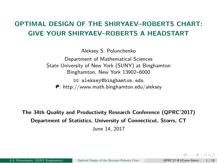
OPTIMAL DESIGN OF THE SHIRYAEV–ROBERTS CHART: GIVE YOUR SHIRYAEV–ROBERTS A HEADSTART Aleksey S. Polunchenko Department of Mathematical Sciences State University of New York (SUNY) at Binghamton Binghamton, New York 13902–6000 � : aleksey@binghamton.edu � : http://www.math.binghamton.edu/aleksey The 34th Quality and Productivity Research Conference (QPRC’2017) Department of Statistics, University of Connecticut, Storrs, CT June 14, 2017 A.S. Polunchenko (SUNY Binghamton) Optimal Design of the Shiryaev–Roberts Chart QPRC’17 @ UConn–Storrs 1 / 19

b bc b b b bc bc bc bc Quickest change-point detection problem • Given: A series { X n } n ≥ 1 of independent scalar data, collected sequentially, one at a time. { X n } n ≥ 1 independent throughout X 1 X 2 X 3 X ν − 1 X ν X ν +1 X ν +2 X ν +3 X n each X n ∝ f ( x ) each X n ∝ g ( x ) �≡ f ( x ) Change-Point Surveillance Starts ( ν ≥ 0, unknown) Surveillance Continues • Assumption 1: X n ∝ p X n ( x ), where p X n ( x ) = µ 1 l { n >ν } + ǫ n , µ � = 0, and { ǫ n } n � 1 are iid standard Gaussian random variables. • Assumption 2: The change-point, ν � 0, is unknown , but not random (no prior distribution). • Notation: from now on a ) ν = 0 is to be understood as E [ X n ] = µ for all n � 1, and b ) ν = ∞ is to mean that E [ X n ] = 0 for all n � 1. A.S. Polunchenko (SUNY Binghamton) Optimal Design of the Shiryaev–Roberts Chart QPRC’17 @ UConn–Storrs 2 / 19

Minimax change-point detection problem • Notation: let T denote a generic chart (stopping time). • Notation: for k � 0 let P k ( · ) = P ( · | ν = k ) and E k [ · ] = E [ · | ν = k ]; in particular, P ∞ ( · ) = P ( · | ν = ∞ ) and E ∞ [ · ] = E [ · | ν = ∞ ] • Define SADD( T ) = sup 0 ≤ ν< ∞ ADD ν ( T ) with ADD ν ( T ) = E ν [ T − ν | T > ν ], ν � 0. • Define ARL( T ) = E ∞ [ T ]. • Goal: To find stopping time T such that SADD( T ) is minimized within class ∆( γ ) = { T : ARL( T ) � γ } for every γ � 1. • Note: Except for a few special cases, this problem has not yet been solved. • The best available solution is a “tweaked” version of the so-called Shiryaev–Roberts detection procedure, due to Shiryaev (1961’63) and Roberts (1966). A.S. Polunchenko (SUNY Binghamton) Optimal Design of the Shiryaev–Roberts Chart QPRC’17 @ UConn–Storrs 3 / 19

The Shiryaev–Roberts (SR) chart • Introduce the “score-function” S n = µ X n − µ 2 2 , n = 1 , 2 , . . . and define R n = (1 + R n − 1 ) exp { S n } , n = 1 , 2 , . . . , where R 0 = 0. • The classical SR chart calls for stopping at S A = inf { n � 1: R n � A } with A > 0 , where A > 0 is a control limit selected in advance so that ARL( S A ) � γ for a given γ � 1. • Moustakides, P. and Tartakovsky (2011) proposed to parameterize the starting point R 0 = r � 0. One can then define the Generalized SR chart as S r A = inf { n � 1: R r n � A } , where R r n = (1 + R r n − 1 ) exp { S n } . A.S. Polunchenko (SUNY Binghamton) Optimal Design of the Shiryaev–Roberts Chart QPRC’17 @ UConn–Storrs 4 / 19

The GSR chart (cont’d) STATISTICAL INFERENCE X 1 , . . . , X n MAXIMUM LIKELIHOOD APPROACH (GENERALIZED) BAYESIAN APPROACH DECISION STATISTIC OF THE FORM DECISION STATISTIC OF THE FORM max k φ k ( X 1 , . . . , X k ) � k φ k ( X 1 , . . . , X k ) Figure 1. Approaches to statistical inference. A.S. Polunchenko (SUNY Binghamton) Optimal Design of the Shiryaev–Roberts Chart QPRC’17 @ UConn–Storrs 5 / 19

The GSR chart: Properties • Observation: { R r n − n − r } n � 0 is a zero-mean P ∞ -martingale, i.e., E ∞ [ R r n − n − r ] = 0. • Consequence 1: E ∞ [ R r A − S r A − r ] = 0 so that ARL( S r A ) = E ∞ [ R r A ] − r . S r S r • Consequence 2: ARL( S r A ) as a function of r should be almost linear. • Moreover, it can be shown that E ∞ [ R r A ] → A / v as A → ∞ , where v is the limiting S r exponential overshoot. • Hence, ARL( S r A ) is also linear in A . • The linearity of ARL( S r A ) is important in designing a numerical method to compute it. • The GSR procedure is asymptotically (as the ARL to false alarm increases) nearly (order-three) optimal with respect to SADD( T ). That is, SADD( S r A ) = inf T ∈ ∆( γ ) SADD( T ) + o (1), as γ → ∞ , where o (1) → 0, as γ → ∞ . • P. & Tartakovsky (2010) and Tartakovsky & P. (2010) offer two special cases where the GSR procedure is exactly SADD( T )-optimal. A.S. Polunchenko (SUNY Binghamton) Optimal Design of the Shiryaev–Roberts Chart QPRC’17 @ UConn–Storrs 6 / 19

bc bc bc bc bc bc The GSR chart: Choosing the headstart • Let ARL( S r A ) = γ , where γ > 1 is fixed . R 0 = 0 0 < R 0 < r ∗ R 0 ∼ Q A ( x ) R 0 > r ∗ A > ν ] A − ν |S r E ν [ S r R 0 = r ∗ ν Figure 2. ADD ν ( S r A ) as a function of ν and R r 0 = r . A.S. Polunchenko (SUNY Binghamton) Optimal Design of the Shiryaev–Roberts Chart QPRC’17 @ UConn–Storrs 7 / 19

The GSR chart: Choosing the headstart (cont’d) • If we had a lowerbound for SADD( S r A ) as a function of r , then it would make sense to let r to be such that the difference between SADD( S r A ) and the lowerbound is minimized. Theorem If A = A γ so that ARL( S r A γ ) = γ , then for every r � 0 it is true that T ∈ ∆( γ ) SADD( T ) � SADD( S r inf A ) , where � ∞ � � SADD( S r r E 0 [ S r E k [max { 0 , S r / ( r + ARL( S r A ) � A ] + A − k } ] A )) . k =0 • See Moustakides, P. & Tartakovsky (2011), P. & Tartakovsky (2010), Tartakovsky & P. (2010), Pollak & Tartakovsky (2009), and Shiryaev & Zryumov (2010). A.S. Polunchenko (SUNY Binghamton) Optimal Design of the Shiryaev–Roberts Chart QPRC’17 @ UConn–Storrs 8 / 19

The GSR chart: Choosing the headstart (cont’d) • Since SADD( S r A ) � inf T ∈ ∆( γ ) SADD( T ) � SADD( S r A ), the number � � SADD( S r A ) − SADD( S r r opt = arg inf A ) 0 � r < A is a good candidate for the point to start the GSR chart from. • The lowerbound can be conveniently and accurately computed via the numerical framework proposed by P., Sokolov & Du (2014). A.S. Polunchenko (SUNY Binghamton) Optimal Design of the Shiryaev–Roberts Chart QPRC’17 @ UConn–Storrs 9 / 19

Numerical results: ARL to false alarm 1000 1000 1000 900 1000 1000 900 800 1000 900 800 800 700 900 800 600 700 800 900 500 700 600 400 900 800 600 500 700 800 A ) A ) 500 700 600 600 600 400 600 ARL( S r 500 700 ARL( S r 300 800 500 400 600 400 700 600 500 300 300 700 200 500 200 400 600 700 400 400 100 500 400 600 300 300 500 200 200 400 600 400 100 600 300 500 300 500 200 200 400 400 100 100 300 500 300 200 200 200 500 200 400 400 100 300 100 300 200 200 400 400 100 300 100 300 1 1 200 200 100 300 100 300 1000 1000 200 200 100 100 800 800 200 200 1000 1000 100 100 600 600 800 800 100 100 600 600 400 400 400 400 200 200 200 200 0 0 0 Headstart, R r 0 Headstart, R r 0 = r Detection Threshold, A 0 = r Detection Threshold, A (a) µ = 0 . 2. (b) µ = 0 . 5. Figure 3. ARL( S r A ) as a function of the headstart R r 0 = r � 0 and the detection threshold A > 0 for µ = { 0 . 2 , 0 . 5 } . A.S. Polunchenko (SUNY Binghamton) Optimal Design of the Shiryaev–Roberts Chart QPRC’17 @ UConn–Storrs 10 / 19

Numerical results: Average Detection Delay 60 120 140 50 100 120 A ) A ) A ) ADD k ( S r 40 ADD k ( S r ADD k ( S r 80 100 30 60 80 20 10 40 60 0 100 0 250 0 500 80 200 400 50 50 50 60 150 300 100 100 100 40 100 200 150 150 150 20 50 100 Headstart, R r 0 = r Headstart, R r 0 = r Headstart, R r 200 Change-Point, k 200 Change-Point, k 0 = r 200 Change-Point, k 0 0 0 (a) γ = 100. (b) γ = 500. (c) γ = 1 000. Figure 4. ADD k ( S r A ) as a function of the headstart R r 0 = r � 0, the change-point k = 0 , 1 , . . . , and the ARL to false alarm level ARL( S r A ) = γ > 1 for µ = 0 . 2. A.S. Polunchenko (SUNY Binghamton) Optimal Design of the Shiryaev–Roberts Chart QPRC’17 @ UConn–Storrs 11 / 19

Numerical results: Average Detection Delay (cont’d) 25 30 35 20 25 30 A ) A ) A ) ADD k ( S r 15 ADD k ( S r 20 ADD k ( S r 25 10 15 20 5 10 15 0 5 10 0 100 0 100 0 100 80 80 80 50 50 50 60 60 60 100 100 100 40 40 40 150 150 150 20 20 20 Headstart, R r 0 = r Headstart, R r Headstart, R r 0 = r 200 Change-Point, k 0 = r Change-Point, k Change-Point, k 0 200 0 200 0 (a) γ = 100. (b) γ = 500. (c) γ = 1 000. Figure 5. ADD k ( S r A ) as a function of the headstart R r 0 = r � 0, the change-point k = 0 , 1 , . . . , and the ARL to false alarm level ARL( S r A ) = γ > 1 for µ = 0 . 5. A.S. Polunchenko (SUNY Binghamton) Optimal Design of the Shiryaev–Roberts Chart QPRC’17 @ UConn–Storrs 12 / 19